Multiple Linear Regression
IN1002B: Introduction to Data Science Projects
Department of Industrial Engineering
Agenda
- Introduction
- Multiple linear regression model
- Parameter estimation
statsmodels library
- statsmodels is a powerful Python library for statistical modeling, data analysis, and hypothesis testing.
- It provides classes and functions for estimating statistical models.
- It is built on top of libraries such as NumPy, SciPy, and pandas
- https://www.statsmodels.org/stable/index.html
Load the libraries
Let’s import statsmodels into Python together with the other relevant libraries.
Multiple linear regression model
Example
A group of engineers conducted an experiment to determine the influence of five factors on an appropriate measure of the whiteness of rayon (\(Y\)). The factors (predictors) are
- \(X_1\): acid bath temperature.
- \(X_2\): cascade acid concentration.
- \(X_3\): water temperature.
- \(X_4\): sulfide concentration.
- \(X_5\): amount of chlorine bleach.
The dataset
The dataset for the file is in “rayon.xlsx”. It has 26 observations.
| X1 | X2 | X3 | X4 | X5 | Y | |
|---|---|---|---|---|---|---|
| 0 | 35 | 0.3 | 82 | 0.2 | 0.3 | 76.5 |
| 1 | 35 | 0.3 | 82 | 0.3 | 0.5 | 76.0 |
| 2 | 35 | 0.3 | 88 | 0.2 | 0.5 | 79.9 |
| 3 | 35 | 0.3 | 88 | 0.3 | 0.3 | 83.5 |
| 4 | 35 | 0.7 | 82 | 0.2 | 0.5 | 89.5 |
Here, we will consider it as the training dataset.
Multiple linear regression model
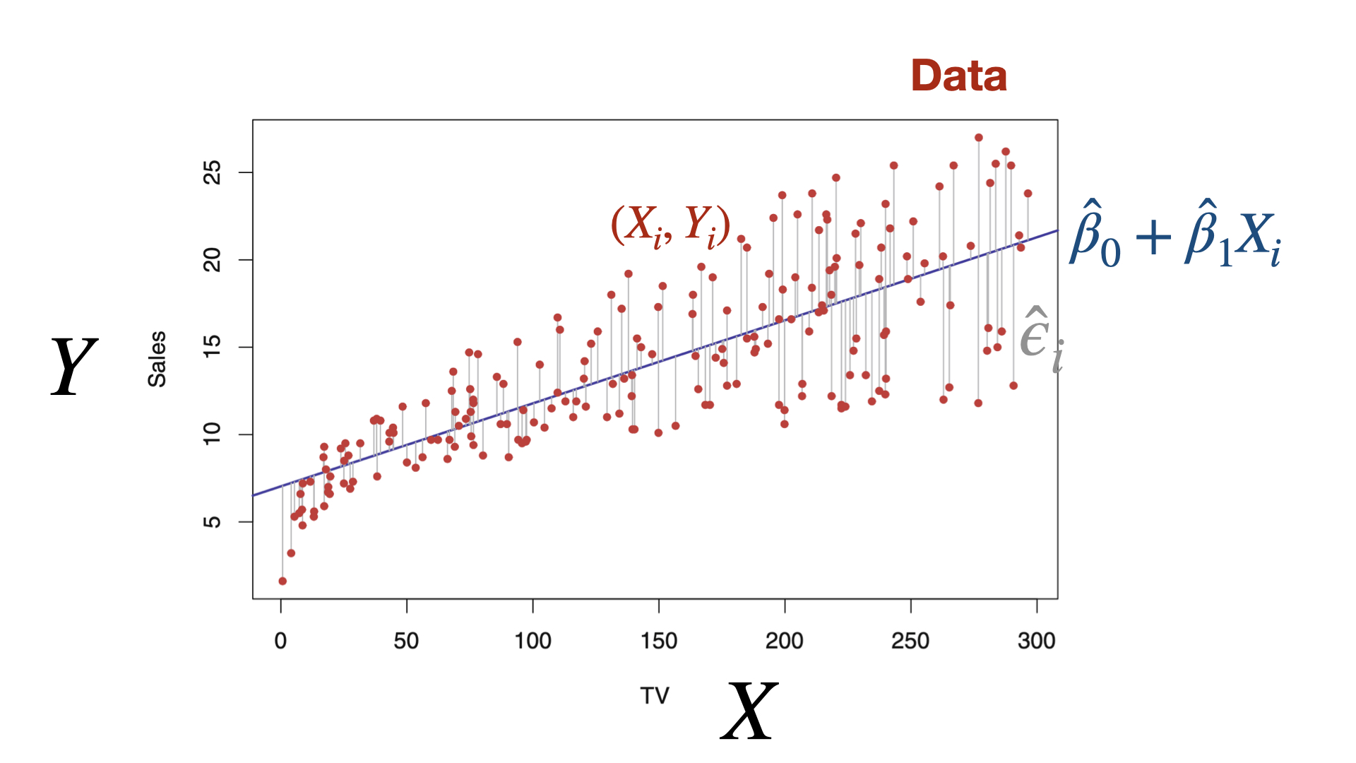
\[Y = f(\boldsymbol{X}) + \epsilon\]
- \(f(\boldsymbol{X}) = \beta_0 + \beta_1 X_1 + \cdots + \beta_p X_p\) (constant).
- \(p\) is the number of predictors.
- \(\epsilon\) is a random variable describing everything that is not captured by our model.
Assumptions:
- The expected or average value of \(\epsilon\) is zero.
- The dispersion or variance of \(\epsilon\) is \(\sigma^2\) (unknown constant).
In our example
\[Y = \beta_0 + \beta_1 X_1 + \beta_2 X_2 + \beta_3 X_3 + \beta_4 X_4 + \beta_5 X_5 + \epsilon\]
\(X_1\): acid bath temperature.
\(X_2\): cascade acid concentration.
\(X_3\): water temperature.
\(X_4\): sulfide concentration.
\(X_5\): amount of chlorine bleach.
\(Y\): whiteness of rayon.
\(p = 5\) and \(\epsilon\) is the error of the model assumed to be 0 and of constant dispersion \(\sigma^2\).
Interpretation of coefficients
\[f(\boldsymbol{X}) = \beta_0 + \beta_1 X_1 + \beta_2 X_2 + \cdots + \beta_p X_p,\]
where the unknown parameter \(\beta_0\) is called the “intercept,” and \(\beta_j\) is the “coefficient” of the j-th predictor.
For the j-th predictor, we have that:
- \(\beta_j = 0\) implies no dependence.
- \(\beta_j > 0\) implies positive dependence.
- \(\beta_j < 0\) implies negative dependence.
\[f(\boldsymbol{X}) = \beta_0 + \beta_1 X_1 + \beta_2 X_2 + \cdots + \beta_p X_p,\]
Interpretation:
- \(\beta_0\) is the average response when all predictors \(X_j\) equal 0.
- \(\beta_j\) is the amount of increase in the average response by a 1 unit increase in the predictor \(X_j\), when all other predictors are fixed to an arbitrary value.
Training Data
The parameters \(\beta_0, \beta_1, \ldots, \beta_p\) and \(\sigma^2\) are unknown. To learn about them, we use our training data.
| X1 | X2 | X3 | X4 | X5 | Y | |
|---|---|---|---|---|---|---|
| 0 | 35 | 0.3 | 82 | 0.2 | 0.3 | 76.5 |
| 1 | 35 | 0.3 | 82 | 0.3 | 0.5 | 76.0 |
| 2 | 35 | 0.3 | 88 | 0.2 | 0.5 | 79.9 |
| 3 | 35 | 0.3 | 88 | 0.3 | 0.3 | 83.5 |
| 4 | 35 | 0.7 | 82 | 0.2 | 0.5 | 89.5 |
Notation
- \(X_{ij}\) denotes the i-th observed value of predictor \(X_j\).
- \(Y_i\) denotes the i-th observed value of response \(Y\).
| X1 | X2 | X3 | X4 | X5 | Y | |
|---|---|---|---|---|---|---|
| 0 | 35 | 0.3 | 82 | 0.2 | 0.3 | 76.5 |
| 1 | 35 | 0.3 | 82 | 0.3 | 0.5 | 76.0 |
| 2 | 35 | 0.3 | 88 | 0.2 | 0.5 | 79.9 |
| 3 | 35 | 0.3 | 88 | 0.3 | 0.3 | 83.5 |
| 4 | 35 | 0.7 | 82 | 0.2 | 0.5 | 89.5 |
Since we believe in the multiple linear regression model, then the observations in the data set must comply with
\[Y_i= \beta_0+\beta_1 X_{i1} + \beta_2 X_{i2} + \cdots + \beta_p X_{ip} + \epsilon_i.\]
where:
\(i=1, \ldots, n.\)
\(n\) is the number of observations. In our example, \(n = 26\).
The \(\epsilon_1, \epsilon_2, \ldots, \epsilon_n\) are random errors.
Assumptions of the errors
\[Y_i= \beta_0+\beta_1 X_{i1} + \beta_2 X_{i2} + \cdots + \beta_p X_{ip} + \epsilon_i \]
The error \(\epsilon_i\)’s must satisfy the following assumptions:
- On average, they are close to zero for any values of the predictors \(X_j\).
- For any value of a predictor \(X_i\), the dispersion or variance is constant and equal to \(\sigma^2\).
- The \(\epsilon_i\)’s are all independent from each other.
- The \(\epsilon_i\)’s follow normal distribution with mean 0 and variance \(\sigma^2\).
Questions
How can we estimate \(\beta_0, \beta_1, \ldots, \beta_p\) and \(\sigma^2\)?
How can we validate the model and all its assumptions?
How can we make inferences about \(\beta_0, \beta_1, \ldots, \beta_p\)?
If some assumptions are not met, can we do something about it?
How can we make predictions of future responses using the multiple linear regression model?
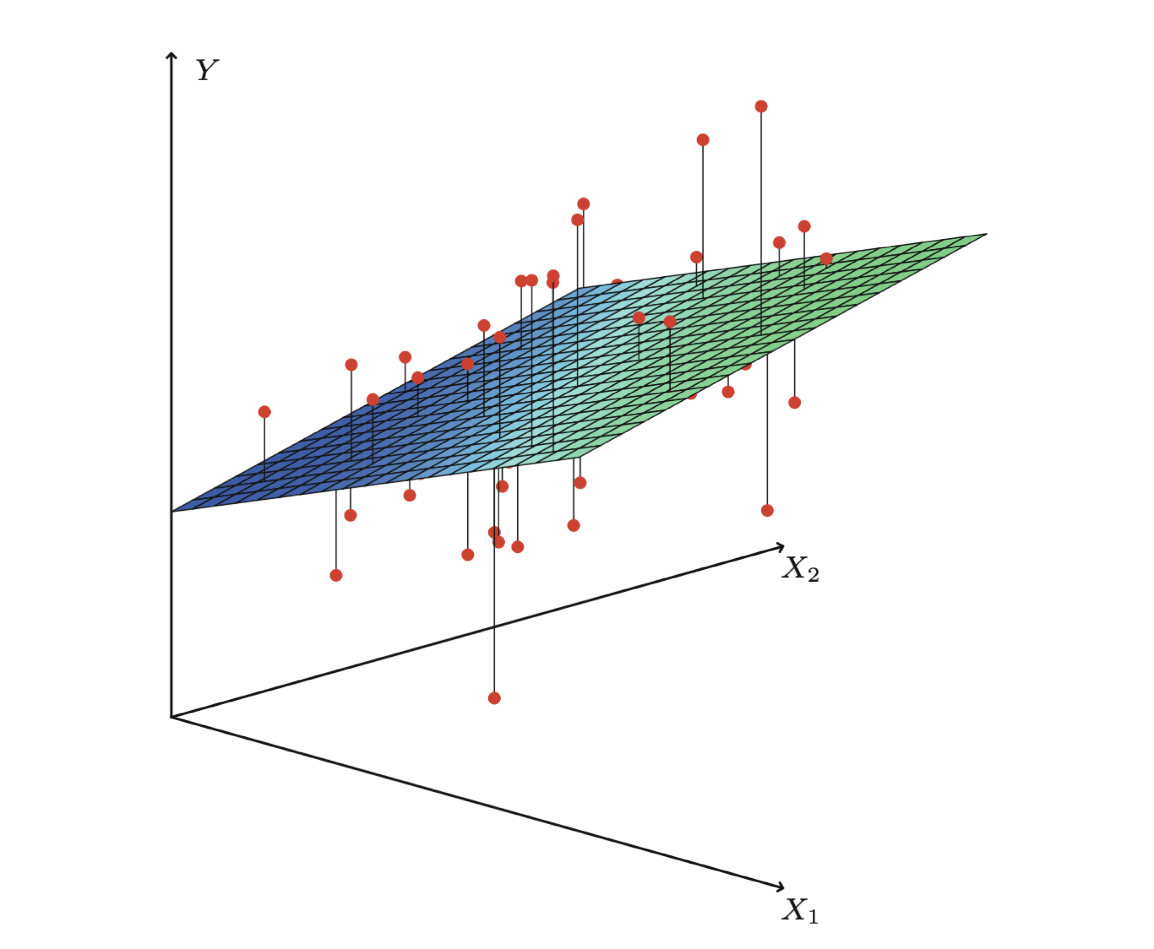
Matrix notation
In what follows, it is useful to denote the multiple linear regression model using matrix notation:
\(\mathbf{Y} = \begin{pmatrix} Y_1 \\ Y_2 \\ \vdots \\ Y_n \end{pmatrix}\) and \(\mathbf{X} = \begin{pmatrix} 1& X_{11} & X_{12} & \cdots & X_{1p} \\ 1& X_{21} & X_{22} & \cdots & X_{2p} \\ \vdots &\vdots & \vdots & \cdots & \vdots \\ 1& X_{n1} & X_{n2} & \cdots & X_{np} \\ \end{pmatrix}\), where
- \(\mathbf{Y}\) is an \(n \times 1\) vector.
- \(\mathbf{X}\) is a \(n \times (p+1)\) matrix.
And,
\(\boldsymbol{\beta} = \begin{pmatrix}\beta_0 \\ \beta_1 \\ \vdots \\ \beta_p \end{pmatrix}\) and \(\boldsymbol{\epsilon} = \begin{pmatrix}\epsilon_1 \\ \epsilon_2 \\ \vdots \\ \epsilon_n \end{pmatrix}\), where
- \(\boldsymbol{\beta}\) is an \((p+1) \times 1\) vector.
- \(\boldsymbol{\epsilon}\) is an \(n \times 1\) vector.
The multiple linear regression model then is
\[\mathbf{Y} = \mathbf{X}\boldsymbol{\beta} + \boldsymbol{\epsilon}.\] This expression means
\(\begin{pmatrix} Y_1 \\ Y_2 \\ \vdots \\ Y_n \end{pmatrix} = \begin{pmatrix} \beta_0 + \beta_1 X_{11} + \beta_2 X_{12} + \cdots + \beta_p X_{1p} \\ \beta_0 + \beta_1 X_{21} + \beta_2 X_{22} + \cdots + \beta_p X_{2p} \\ \vdots \\ \beta_0 + \beta_1 X_{n1} + \beta_2 X_{n2} + \cdots + \beta_p X_{np} \\ \end{pmatrix} + \begin{pmatrix}\epsilon_1 \\ \epsilon_2 \\ \vdots \\ \epsilon_n \end{pmatrix}\)
Parameter Estimation
Questions
How can we estimate \(\beta_0, \beta_1, \ldots, \beta_p\) and \(\sigma^2\)?
How can we validate the model and all its assumptions?
How can we make inferences about \(\beta_0, \beta_1, \ldots, \beta_p\)?
If some assumptions are not met, can we do something about it?
How can we make predictions of future responses using the multiple linear regression model?
An estimator for \(\boldsymbol{\beta}\)
Our goal is to find an estimator for the vector \(\boldsymbol{\beta}\) (and all its components). For the moment, let’s assume that we have one:
\(\hat{\boldsymbol{\beta}} = \begin{pmatrix} \hat{\beta}_0 \\ \hat{\beta}_1 \\ \vdots\\ \hat{\beta}_p \end{pmatrix}\), where \(\hat{\beta}_j\) is an estimator for \(\beta_j\), \(j = 0, \ldots, p\).
Using this estimator, we can compute the predicted responses of our model \(\hat{\mathbf{Y}} = \mathbf{X}\hat{\boldsymbol{\beta}}\), where \(\hat{\mathbf{Y}} = (\hat{Y}_1, \hat{Y}_2, \ldots, \hat{Y}_n)^{T}\) and \(\hat{Y}_i\) is the i-th predicted response.
The expression \(\hat{\mathbf{Y}} = \mathbf{X}\hat{\boldsymbol{\beta}}\) means
\[\begin{pmatrix} \hat{Y}_1 \\ \hat{Y}_2 \\ \vdots \\ \hat{Y}_n \end{pmatrix} = \begin{pmatrix} \hat{\beta}_0 + X_{11} \hat{\beta}_1 + X_{12} \hat{\beta}_2 + \cdots + X_{1p} \hat{\beta}_p\\ \hat{\beta}_0 + X_{21} \hat{\beta}_1 + X_{22}\hat{\beta}_2 + \cdots + X_{2p}\hat{\beta}_p \\ \vdots \\ \hat{\beta}_0 + X_{n1} \hat{\beta}_1 + X_{n2}\hat{\beta}_2 + \cdots + X_{np} \hat{\beta}_p \\ \end{pmatrix}\]
This means that the residuals of the estimated model are
\[\hat{\boldsymbol{\epsilon}} = \mathbf{Y} - \hat{\mathbf{Y}} = \mathbf{Y} - \mathbf{X} \hat{\boldsymbol{\beta}},\]
where \(\hat{\boldsymbol{\epsilon}} = (\hat{\epsilon}_1, \hat{\epsilon}_2, \ldots, \hat{\epsilon}_n)^{T}\) and \(\hat{\epsilon}_i = Y_i - \hat{Y}_i\) is the i-th residual.
Least squares estimator
To find the best estimator for \(\boldsymbol{\beta}\) (and all its elements), we use the method of least squares. This method finds the best \(\hat{\boldsymbol{\beta}}\) that minimizes the residual sum of squares (RSS):
\[RSS = \left(\mathbf{Y} - \mathbf{X} \hat{\boldsymbol{\beta}}\right)^{T} \left(\mathbf{Y} - \mathbf{X} \hat{\boldsymbol{\beta}}\right) = \sum_{i=1}^{n} \hat{\epsilon}^2_i = \sum_{i=1}^{n} (Y_i - \hat{Y}_i)^2.\]
The estimator that minimizes the expression above is called the least squares estimator:
\[\hat{\boldsymbol{\beta}} = (\mathbf{X}^{T}\mathbf{X})^{-1} \mathbf{X}^{T}\mathbf{Y}\]
Computation of \(\hat{\boldsymbol{\beta}} = (\mathbf{X}^{T}\mathbf{X})^{-1} \mathbf{X}^{T}\mathbf{Y}\)
- Compute the transpose of a matrix: \(\mathbf{X}^{T}\).
- Compute the product of a matrix and a vector: \(\mathbf{X}^{T}\mathbf{Y}\).
- Compute the product of two matrices: \(\mathbf{X}^{T} \mathbf{X}\).
- Compute the inverse of a matrix: \((\mathbf{X}^{T} \mathbf{X})^{-1}\).
Remarks
- Compute the inverse of a matrix: \((\mathbf{X}^{T} \mathbf{X})^{-1}\).
- Not all matrices have an inverse.
- If it does not have an inverse then the matrix is called singular. Otherwise, it is called non-singular.
- For the inverse to exist, the columns in \(\mathbf{X}\) must be linearly independent.
- Or, equivalently, the determinant \(|\mathbf{X}^{T} \mathbf{X}| > 0\).
Computation in Python
To compute the least squares estimates, we first split the data set into a matrix with the values of the predictors only, and a matrix with the response values.
Next, we use the functions OLS() and fit() from statsmodels.
To show the estimated coefficients, we use the argument params of the linear_model object created previously.
const   -35.262607
X1        0.745417
X2       20.229167
X3        0.793056
X4       25.583333
X5       17.208333
dtype: float64
The elements in the vector above are the estimates \(\hat{\beta}_0\), \(\hat{\beta}_1\), \(\hat{\beta}_2\), \(\hat{\beta}_3\), \(\hat{\beta}_4\), and \(\hat{\beta}_5\).
Interpretation of estimated coefficients
The average whiteness of a rayon is \(\hat{\beta}_0 = -35.26\) when all predictors are equal to 0.
Increasing the acid bath temperature by 1 unit increases the average whiteness of a rayon by \(\hat{\beta}_1 = 0.745\) units.
Increasing the cascade acid concentration by 1 unit increases the average whiteness of a rayon by \(\hat{\beta}_2 = 20.23\) units.
Increasing the water temperature by 1 unit increases the average whiteness of a rayon by \(\hat{\beta}_3 = 0.793\) units.
Increasing the sulfide concentration by 1 unit increases the average whiteness of a rayon by \(\hat{\beta}_4 = 25.583\) units.
Increasing the amount of chlorine bleach by 1 unit increases the average whiteness of a rayon by \(\hat{\beta}_5 = 17.208\) units.
Properties of least squares estimators
If all the assumptions of the linear regression model are met, the least squares estimators have some attractive properties.
For example:
- On average, the estimate \(\hat{\beta}_{j}\) equals the true coefficient value \(\beta_{j}\) for the predictor \(X_j\).
- Each estimate \(\hat{\beta}_{j}\) follows a normal distribution with a specific mean and variance.
Predictions
Once we estimate the intercept and model coefficients, we make predictions as follows:
\[\hat{Y}_i = \hat{\beta}_0 + \hat{\beta}_1 X_{i1} + \hat{\beta}_2 X_{i2} + \cdots + \hat{\beta}_p X_{ip}\]
where \(\hat{Y}_i\) is the i-th fitted or predicted response.
In Python, we use the argument fittedvalues to show the predicted responses of the estimated model.
Predictions of the 26 observations in the training dataset.
0      72.205449
1      78.205449
2      80.405449
3      79.522115
4      83.738782
5      82.855449
6      85.055449
7      91.055449
8      90.555449
9      89.672115
10     91.872115
11     97.872115
12     95.205449
13    101.205449
14    103.405449
15    102.522115
16     74.176282
17    103.992949
18     80.992949
19     97.176282
20     84.326282
21     93.842949
22     86.526282
23     91.642949
24     85.642949
25     92.526282
dtype: float64
Residuals
Now that we have introduced the estimator \(\hat{\beta}_0, \hat{\beta}_1, \ldots, \hat{\beta}_p\), we can be more specific in our terminology of the linear model.
The errors of the estimated model are called residuals \(\hat{\epsilon}_i = Y_i - \hat{Y}_i\), \(i = 1, \ldots, n.\)
If the model is correct, the residuals \(\hat{\epsilon}_1, \hat{\epsilon}_2, \ldots, \hat{\epsilon}_n\) give us a good idea of the errors \(\epsilon_1, \epsilon_2, \ldots, \epsilon_n\).
In Python, we compute the residuals using the following command.
0      4.294551
1     -2.205449
2     -0.505449
3      3.977885
4      5.761218
5      1.344551
6      0.644551
7      8.444551
8     -1.155449
9      7.827885
10    11.327885
11    10.827885
12    19.994551
13    10.294551
14    -1.105449
15     5.577885
16     6.023718
17   -14.892949
18    -3.792949
19   -12.076282
20   -12.826282
21    -9.342949
22    -9.026282
23   -12.442949
24   -14.642949
25    -2.326282
dtype: float64
Estimation of variance
The variance \(\sigma^2\) of the errors is estimated by
\[\hat{\sigma}^2=\frac{1}{n-p-1}\sum_{i=1}^{n} \hat{\epsilon}_i^{2},\]
where \(n\) and \(p\) are the numbers of observations and predictors, respectively. In Python, we compute \(\hat{\sigma}^2\) as follows:
The smaller the value of \(\hat{\sigma}^2\), the closer our predictions are to the actual responses.
In practice, it is better to use the standard deviation of the errors. That is,
\[\hat{\sigma}=\left(\frac{1}{n-p-1}\sum_{i=1}^{n} \hat{\epsilon}_i^{2}\right)^{1/2}.\] In Python, we compute \(\hat{\sigma}\) as follows:
Interpretation of \(\hat{\sigma}\)
- The smaller the \(\hat{\sigma}\), the closer our predictions are to the actual responses in the training dataset.
- The \(\hat{\sigma} = 10.292\) implies that, on average, the predictions of our model are off or incorrect by 10.292 units.
Return to main page
![]()
Tecnologico de Monterrey