import pandas as pd
import matplotlib.pyplot as plt
import seaborn as sns
from sklearn.model_selection import train_test_split
from sklearn.impute import SimpleImputer, KNNImputer
from sklearn.preprocessing import PowerTransformer, StandardScaler
from sklearn.feature_selection import VarianceThresholdData preprocessing: Part I
IN1002B: Introduction to Data Science Projects
Alan R. Vazquez
Department of Industrial Engineering
Agenda
- Introduction
- Training, validation, and test datasets
- Dealing with missing values
Introduction
Data preprocessing
Data pre-processing techniques generally refer to the addition, deletion, or transformation of data.
It can make or break a model’s predictive ability.
For example, linear regression models (to be discussed later) are relatively insensitive to the characteristics of the predictor data, but advanced methods like K-nearest neighbors, principal component regression, and LASSO are not.
We will review some common strategies for processing predictors from the data, without considering how they might be related to the response.
In particular, we will review:
- Dealing with missing values.
- Transforming predictors.
- Reducing the number of predictors.
- Standardizing the units of the predictors.
scikit-learn library
- scikit-learn is a robust and popular library for machine learning in Python
- It provides simple, efficient tools for data mining and data analysis
- It is built on top of libraries such as NumPy, SciPy, and Matplotlib
- https://scikit-learn.org/stable/

Let’s import scikit-learn into Python together with the other relevant libraries.
We will not use all the functions from the scikit-learn library. Instead, we will use specific functions from the sub-libraries preprocessing, feature_selection, model_selection and impute.
Training, validation, and test datasets
Recall that …
In data science, we assume that
\[Y = f(\boldsymbol{X}) + \epsilon\]
where \(f(\boldsymbol{X})\) represents the true relationship between \(\boldsymbol{X} = (X_1, X_2, \ldots, X_p)\) and \(Y\).
- \(f(\boldsymbol{X})\) is unknown and very complex!
Two datasets
The application of data science models needs two data sets:
Training data is data that we use to train or construct the estimated function \(\hat{f}(\boldsymbol{X})\).
Test data is data that we use to evaluate the predictive performance of \(\hat{f}(\boldsymbol{X})\) only.

A random sample of \(n\) observations.
Use it to construct \(\hat{f}(\boldsymbol{X})\).

Another random sample of \(n_t\) observations, which is independent of the training data.
Use it to evaluate \(\hat{f}(\boldsymbol{X})\).
Validation Dataset
In many practical situations, a test dataset is not available. To overcome this issue, we use a validation dataset.
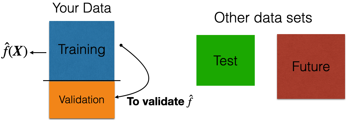
Idea: Apply model to your validation dataset to mimic what will happen when you apply it to test dataset.
Example 1
The “BostonHousing.xlsx” contains data collected by the US Bureau of the Census concerning housing in the area of Boston, Massachusetts. The dataset includes data on 506 census housing tracts in the Boston area in 1970s.
The goal is to predict the median house price in new tracts based on information such as crime rate, pollution, and number of rooms.
The response is the median value of owner-occupied homes in $1000s, contained in the column MEDV.
The predictors
CRIM: per capita crime rate by town.ZN: proportion of residential land zoned for lots over 25,000 sq.ft.INDUS: proportion of non-retail business acres per town.CHAS: Charles River (‘Yes’ if tract bounds river; ‘No’ otherwise).NOX: nitrogen oxides concentration (parts per 10 million).RM: average number of rooms per dwelling.AGE: proportion of owner-occupied units built prior to 1940.DIS: weighted mean of distances to five Boston employment centersRAD: index of accessibility to radial highways (‘Low’, ‘Medium’, ‘High’).TAX: full-value property-tax rate per $10,000.PTRATIO: pupil-teacher ratio by town.LSTAT: lower status of the population (percent).
Read the dataset
We read the dataset and set the variable CHAS and RAD as categorical.
| CRIM | ZN | INDUS | CHAS | NOX | RM | AGE | DIS | RAD | TAX | PTRATIO | LSTAT | MEDV | |
|---|---|---|---|---|---|---|---|---|---|---|---|---|---|
| 0 | 0.00632 | 18.0 | 2.31 | No | 0.538 | 6.575 | 65.2 | 4.0900 | Low | 296 | 15.3 | 4.98 | 24.0 |
| 1 | 0.02731 | 0.0 | 7.07 | No | 0.469 | 6.421 | 78.9 | 4.9671 | Low | 242 | 17.8 | 9.14 | 21.6 |
| 2 | 0.02729 | 0.0 | 7.07 | No | 0.469 | 7.185 | 61.1 | 4.9671 | Low | 242 | 17.8 | 4.03 | 34.7 |
| 3 | 0.03237 | 0.0 | 2.18 | No | 0.458 | 6.998 | 45.8 | 6.0622 | Low | 222 | 18.7 | 2.94 | 33.4 |
| 4 | 0.06905 | 0.0 | 2.18 | No | 0.458 | 7.147 | 54.2 | 6.0622 | Low | 222 | 18.7 | 5.33 | 36.2 |
How do we generate validation data?
We split the current dataset into a training and a validation dataset. To this end, we use the function train_test_split() from scikit-learn.
The function has three main inputs:
- A pandas dataframe with the predictor columns only.
- A pandas dataframe with the response column only.
- The parameter
test_sizewhich sets the portion of the dataset that will go to the validation set.
Create the predictor matrix
We use the function .drop() from pandas. This function drops one or more columns from a data frame. Let’s drop the response column MEDV and store the result in X_full.
| CRIM | ZN | INDUS | CHAS | NOX | RM | AGE | DIS | RAD | TAX | PTRATIO | LSTAT | |
|---|---|---|---|---|---|---|---|---|---|---|---|---|
| 0 | 0.00632 | 18.0 | 2.31 | No | 0.538 | 6.575 | 65.2 | 4.0900 | Low | 296 | 15.3 | 4.98 |
| 1 | 0.02731 | 0.0 | 7.07 | No | 0.469 | 6.421 | 78.9 | 4.9671 | Low | 242 | 17.8 | 9.14 |
| 2 | 0.02729 | 0.0 | 7.07 | No | 0.469 | 7.185 | 61.1 | 4.9671 | Low | 242 | 17.8 | 4.03 |
| 3 | 0.03237 | 0.0 | 2.18 | No | 0.458 | 6.998 | 45.8 | 6.0622 | Low | 222 | 18.7 | 2.94 |
Create the response column
We use the function .filter() from pandas to extract the column MEDV from the data frame. We store the result in Y_full.
Let’s partition the dataset
The function makes a clever partition of the data using the empirical distribution of the response.
Technically, it splits the data so that the distribution of the response under the training and validation sets is similar.
Usually, the proportion of the dataset that goes to the validation set is 20% or 30%.
The predictors and response in the training dataset are in the objects X_train and Y_train, respectively. We compile these objects into a single dataset using the function .concat() from pandas. The argument axis = 1 tells .concat() to concatenate the datasets by their rows.
| CRIM | ZN | INDUS | CHAS | NOX | RM | AGE | DIS | RAD | TAX | PTRATIO | LSTAT | MEDV | |
|---|---|---|---|---|---|---|---|---|---|---|---|---|---|
| 443 | 9.96654 | 0.0 | 18.10 | No | 0.740 | 6.485 | 100.0 | 1.9784 | High | 666 | 20.2 | 18.85 | 15.4 |
| 367 | 13.52220 | 0.0 | 18.10 | No | 0.631 | 3.863 | 100.0 | 1.5106 | High | 666 | 20.2 | 13.33 | 23.1 |
| 93 | 0.02875 | 28.0 | 15.04 | No | 0.464 | 6.211 | 28.9 | 3.6659 | Medium | 270 | 18.2 | 6.21 | 25.0 |
| 247 | 0.19657 | 22.0 | 5.86 | No | 0.431 | 6.226 | 79.2 | 8.0555 | High | 330 | 19.1 | 10.15 | 20.5 |
Equivalently, the predictors and response in the validation dataset are in the objects X_valid and Y_valid, respectively.
| CRIM | ZN | INDUS | CHAS | NOX | RM | AGE | DIS | RAD | TAX | PTRATIO | LSTAT | MEDV | |
|---|---|---|---|---|---|---|---|---|---|---|---|---|---|
| 225 | 0.52693 | 0.0 | 6.20 | No | 0.504 | 8.725 | 83.0 | 2.8944 | High | 307 | 17.4 | 4.63 | 50.0 |
| 33 | 1.15172 | 0.0 | 8.14 | No | 0.538 | 5.701 | 95.0 | 3.7872 | Medium | 307 | 21.0 | 18.35 | 13.1 |
| 72 | 0.09164 | 0.0 | 10.81 | No | 0.413 | 6.065 | 7.8 | 5.2873 | Medium | 305 | 19.2 | 5.52 | 22.8 |
| 7 | 0.14455 | 12.5 | 7.87 | No | 0.524 | 6.172 | 96.1 | 5.9505 | Medium | 311 | 15.2 | 19.15 | 27.1 |
| 340 | 0.06151 | 0.0 | 5.19 | No | 0.515 | 5.968 | 58.5 | 4.8122 | Medium | 224 | 20.2 | 9.29 | 18.7 |
Work on your training dataset
After we have partitioned the data, we work on the training data to develop our predictive pipeline.
The pipeline has two main steps:
- Data preprocessing.
- Model development.
We will now discuss preprocessing techniques applied to the predictor columns in the training dataset.
Note that all preprocessing techniques will also be applied to the validation dataset and test dataset to prepare it for your model!
Dealing with missing values
Missing values
In many cases, some predictors have no values for a given observation. It is important to understand why the values are missing.
There four main types of missing data:
Structurally missing data is data that is missing for a logical reason or because it should not exist.
Missing completely at random assumes that the fact that the data is missing is unrelated to the other information in the data.
Missing at random assumes that we can predict the value that is missing based on the other available data.
Missing not at random assumes that there is a mechanism that generates the missing values, which may include observed and unobserved predictors.
For large data sets, removal of observations based on missing values is not a problem, assuming that the type of missing data is completely at random.
In a smaller data sets, there is a high price in removing observations. To overcome this issue, we can use methods of imputation, which try to estimate the missing values of a predictor variable using the other predictors’ values.
Here, we will introduce some simple methods for imputing missing values in categorical and numerical variables.
Example 2
Let’s use the penguins dataset available in the file “penguins.xlsx”.
# Load the Excel file into a pandas DataFrame.
penguins_data = pd.read_excel("penguins.xlsx")

# Set categorical variables.
penguins_data['sex'] = pd.Categorical(penguins_data['sex'])
penguins_data['species'] = pd.Categorical(penguins_data['species'])
penguins_data['island'] = pd.Categorical(penguins_data['island'])
Training and validation datasets
For illustrative purposes, we assume that we want to predict the species (in the column species) of a penguin using the predictors bill_length_mm, bill_depth_mm, flipper_length_mm, body_mass_g, and sex.
We create the predictor matrix and response column.
We use a validation dataset with 30% of the observations in penguins_data. The other 70% will be in the training dataset.
In train_test_split, we use the input random_state to set a random seed. Essentially, this allows you to obtain the same training and validation datasets every time you run the code. The advice is setting random_state to a big integer number generated at random.
Since preprocessing techniques are meant for the predictors, we will work on the X_train_p data frame.
| bill_length_mm | bill_depth_mm | flipper_length_mm | body_mass_g | sex | |
|---|---|---|---|---|---|
| 31 | 37.2 | 18.1 | 178.0 | 3900.0 | male |
| 46 | 41.1 | 19.0 | 182.0 | 3425.0 | male |
| 195 | 49.6 | 15.0 | 216.0 | 4750.0 | male |
| 43 | 44.1 | 19.7 | 196.0 | 4400.0 | male |
| 196 | 50.5 | 15.9 | 222.0 | 5550.0 | male |
Let’s check if the dataset has missing observations using the function .info() from pandas.
<class 'pandas.core.frame.DataFrame'>
Index: 240 entries, 31 to 293
Data columns (total 5 columns):
 #   Column             Non-Null Count  Dtype
---  ------             --------------  -----
 0   bill_length_mm     238 non-null    float64
 1   bill_depth_mm      238 non-null    float64
 2   flipper_length_mm  238 non-null    float64
 3   body_mass_g        238 non-null    float64
 4   sex                232 non-null    category
dtypes: category(1), float64(4)
memory usage: 9.7 KB
In the output of the function, “non-null” refers to the number of entries in a column that have actual values. That is, the number of entries where there are not NaN.
<class 'pandas.core.frame.DataFrame'>
Index: 240 entries, 31 to 293
Data columns (total 5 columns):
 #   Column             Non-Null Count  Dtype
---  ------             --------------  -----
 0   bill_length_mm     238 non-null    float64
 1   bill_depth_mm      238 non-null    float64
 2   flipper_length_mm  238 non-null    float64
 3   body_mass_g        238 non-null    float64
 4   sex                232 non-null    category
dtypes: category(1), float64(4)
memory usage: 9.7 KB
The “Index” section shows the number of observations in the dataset.
The output below shows that there are 240 entries but bill_length_mm has 238 that are “non-null”. Therefore, this column has two missing observations.
<class 'pandas.core.frame.DataFrame'>
Index: 240 entries, 31 to 293
Data columns (total 5 columns):
 #   Column             Non-Null Count  Dtype
---  ------             --------------  -----
 0   bill_length_mm     238 non-null    float64
 1   bill_depth_mm      238 non-null    float64
 2   flipper_length_mm  238 non-null    float64
 3   body_mass_g        238 non-null    float64
 4   sex                232 non-null    category
dtypes: category(1), float64(4)
memory usage: 9.7 KB
The same is true for the other predictors except for sex that has eight missing values.
Alternatively, we can use the function .isnull() together with sum() to determine the number of missing values for each column in the dataset.
Removing missing values
If we want to remove all rows in the dataset that have at least one missing value, we use the function .dropna().
<class 'pandas.core.frame.DataFrame'>
Index: 232 entries, 31 to 293
Data columns (total 5 columns):
 #   Column             Non-Null Count  Dtype
---  ------             --------------  -----
 0   bill_length_mm     232 non-null    float64
 1   bill_depth_mm      232 non-null    float64
 2   flipper_length_mm  232 non-null    float64
 3   body_mass_g        232 non-null    float64
 4   sex                232 non-null    category
dtypes: category(1), float64(4)
memory usage: 9.4 KB
The new data is complete because each column has 232 “non-null” values; the total number of observations in complete_predictors.
However, note that we have lost eight of the original observations in X_train_p!
Imputation using the mean
We can impute the missing values of a numeric variable using the mean or median of its available values. For example, consider the variable bill_length_mm that has two missing values.
<class 'pandas.core.series.Series'>
Index: 240 entries, 31 to 293
Series name: bill_length_mm
Non-Null Count  Dtype
--------------  -----
238 non-null    float64
dtypes: float64(1)
memory usage: 3.8 KB
In scikit-learn, we use the function SimpleImputer() to define the method of imputation of missing values.
Using SimpleImputer(), we set the method to impute missing values using the mean.
We also use the function fit_transform() to apply the imputation method to the variable.
After imputation, the information of the predictors in the dataset looks like this.
<class 'pandas.core.frame.DataFrame'>
Index: 240 entries, 31 to 293
Data columns (total 5 columns):
 #   Column             Non-Null Count  Dtype
---  ------             --------------  -----
 0   bill_length_mm     240 non-null    float64
 1   bill_depth_mm      238 non-null    float64
 2   flipper_length_mm  238 non-null    float64
 3   body_mass_g        238 non-null    float64
 4   sex                232 non-null    category
dtypes: category(1), float64(4)
memory usage: 9.7 KB
Now, bill_length_mm has 240 complete values.
To impute the missing values using the median, we simply set this method in SimpleImputer(). For example, let’s impute the missing values of bill_depth_mm.
# Imputation for numerical variables (using the mean)
num_imputer = SimpleImputer(strategy = 'median')

# Replace the original variable with new version.
X_train_p['bill_depth_mm'] = num_imputer.fit_transform(X_train_p[ ['bill_depth_mm'] ] )

# Show the information of the predictor.
X_train_p['bill_depth_mm'].info()
<class 'pandas.core.series.Series'>
Index: 240 entries, 31 to 293
Series name: bill_depth_mm
Non-Null Count Dtype
-------------- -----
240 non-null float64
dtypes: float64(1)
memory usage: 3.8 KBUsing the mean or the median?
We use the sample mean when the data distribution is roughly symmetrical.
Pros: Simple and easy to implement.
Cons: Sensitive to outliers; may not be accurate for skewed distributions
We use the sample median when the data is skewed (e.g., incomes, prices).
Pros: Less sensitive to outliers; robust for skewed distributions.
Cons: May reduce variability in the data.
Imputation method for a categorical variable
If a categorical variable has missing values, we can use the most frequent of the available values to replace the missing values. To this end, we use similar commands as before.
For example, let’s impute the missing values of sex using this strategy.
Let’s now have a look at the information of the dataset.
<class 'pandas.core.frame.DataFrame'>
Index: 240 entries, 31 to 293
Data columns (total 5 columns):
 #   Column             Non-Null Count  Dtype
---  ------             --------------  -----
 0   bill_length_mm     240 non-null    float64
 1   bill_depth_mm      240 non-null    float64
 2   flipper_length_mm  238 non-null    float64
 3   body_mass_g        238 non-null    float64
 4   sex                240 non-null    object
dtypes: float64(4), object(1)
memory usage: 11.2+ KB
The columns bill_length_mm, bill_depth_mm, and sex have 240 complete values.
Unfortunately, after applying cat_imputer to the dataset, the variable sex is an object. To change it to categorical, we use the function pd.Categorical again.
# Apply imputation strategy for categorical variables.
X_train_p['sex'] = pd.Categorical(X_train_p['sex'])
X_train_p.info()
<class 'pandas.core.frame.DataFrame'>
Index: 240 entries, 31 to 293
Data columns (total 5 columns):
# Column Non-Null Count Dtype
--- ------ -------------- -----
0 bill_length_mm 240 non-null float64
1 bill_depth_mm 240 non-null float64
2 flipper_length_mm 238 non-null float64
3 body_mass_g 238 non-null float64
4 sex 240 non-null category
dtypes: category(1), float64(4)
memory usage: 9.7 KBMultivariate imputation using K-nearest neighbours
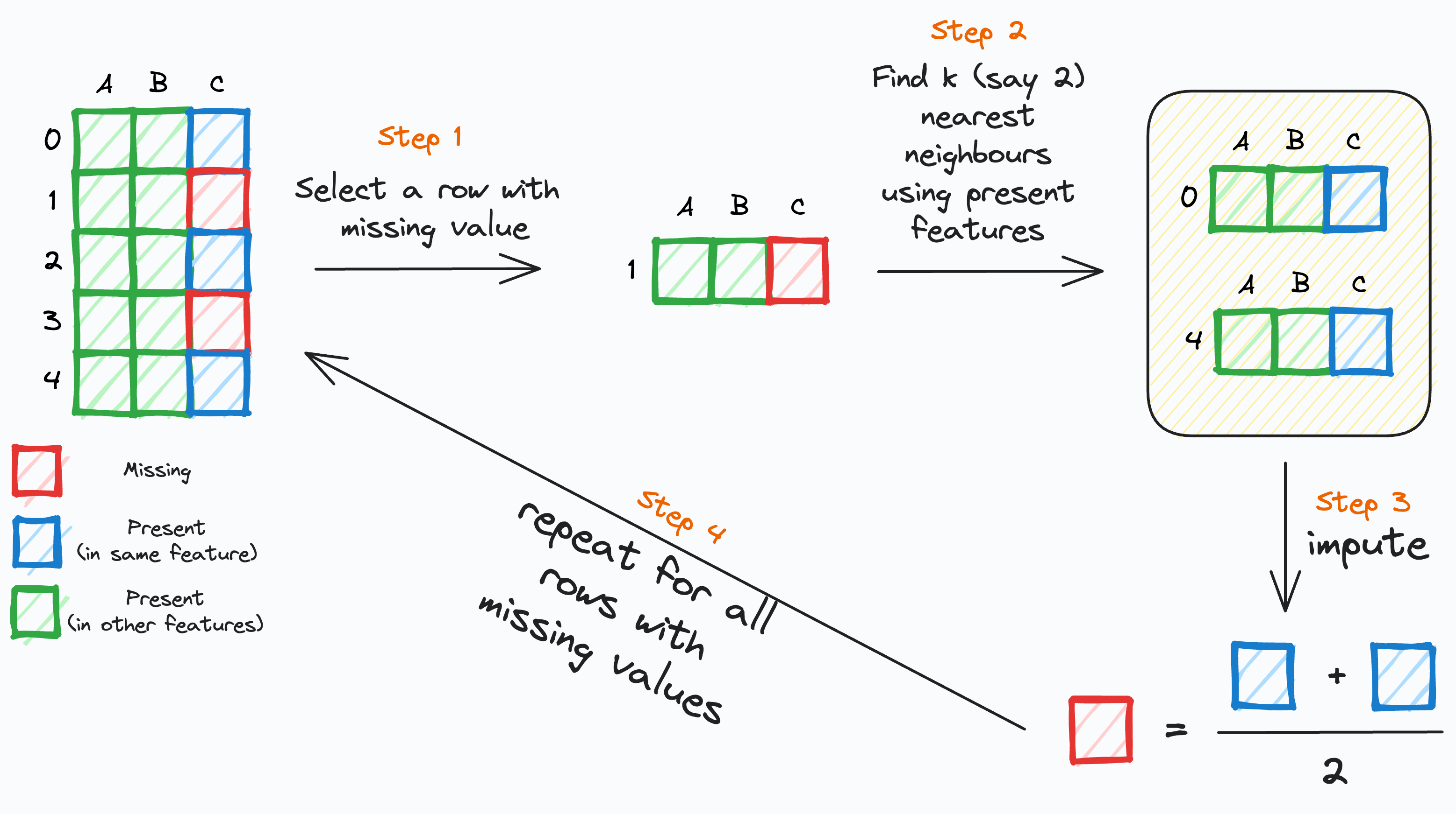
K-nearest neighbours (KNN) is an imputation method to fill in the missing values of a predictor using the available values from this and the other predictors.
For each missing value in a predictor \(X\):
- Find the \(K\) most similar rows based on the other predictors.
- Impute the missing value of \(X\) using the average of the available values of \(X\) in the \(K\) closest rows.
Basic idea
Notes on its implementation
KNN captures local patterns better than individual predictor imputation using the mean or the median.
However, it only works for numeric predictors!
The distance between two rows is calculated using Euclidean distance.
KNN only considers rows without missing values in the predictor columns being used.
In Python
You can use KNN using the function KNNImputer(). Its main input is the number of nearest neighbours to use. You set this value using the parameter n_neighbors.
# Set the KNN imputer using two neighbours.
KNN_imputer = KNNImputer(n_neighbors = 2)

# Select numeric predictors.
X_train_num_p = X_train_p.drop(columns = ['sex'])

# Apply imputer and store the rulst in a pandas data frame.
X_train_num_p = pd.DataFrame(KNN_imputer.fit_transform(X_train_num_p),
                            columns = X_train_num_p.columns)
Let’s look at the new dataset.
<class 'pandas.core.frame.DataFrame'>
RangeIndex: 240 entries, 0 to 239
Data columns (total 4 columns):
 #   Column             Non-Null Count  Dtype
---  ------             --------------  -----
 0   bill_length_mm     240 non-null    float64
 1   bill_depth_mm      240 non-null    float64
 2   flipper_length_mm  240 non-null    float64
 3   body_mass_g        240 non-null    float64
dtypes: float64(4)
memory usage: 7.6 KB
All predictors have 240 complete entries.
Return to main page
![]()
Tecnologico de Monterrey