Introduction to Python and Pandas
IN1002B: Introduction to Data Science Projects
Department of Industrial Engineering
Agenda
- Introduction to Python
- Reading data with Python
Introduction to Python
Python
A versatile programming language.
It is free!
It is widely used for data cleaning, data visualization, and data modelling.
It can be extended with packages (libraries) developed by other users.
Google Colab
Google’s free cloud collaboration platform for creating Python documents.
Run Python and collaborate on Jupyter notebooks for free.
Harness the power of GPUs for free to accelerate your data science projects.
Easily save and upload your notebooks to Google Drive.
Let’s try a command in Python
What do you think will happen if we run this command?
Hello world!Let’s try another command
What do you think will happen if we run this command?
16Use Python as a basic calculator
Introduction to functions in Python
One of the best things about Python is that there are many built-in commands you can use. These are called functions.
Functions have two basic parts:
The first part is the name of the function (for example,
sum).The second part is the input to the function, which goes inside the parentheses (
sum([1, 5, 15])).
Python is strict
Python, like all programming languages, is very strict. For example, if you write
it will tell you the answer, 101.
But if you write
---------------------------------------------------------------------------
NameError                                 Traceback (most recent call last)
Cell In[11], line 1
----> 1 Sum([1, 100])

NameError: name 'Sum' is not defined
with the “s” capitalized, he will act like he has no idea what we are talking about!
Save your work in Python objects
Virtually anything, including the results of any Python function, can be saved in an object.
This is accomplished by using an assignment operator, which can be an equals symbol (=).
You can make up any name you want for a Python object. However, there are two basic rules for this:
- It has to be different from a function name in Python.
- It has to be as specific as possible.
For example
After running this code, nothing happens. But if we run the object on its own, we can see what’s inside it.
You can also use print(my_favorite_number).
Lists
So far we have used Python objects to store a single number. But in statistics we are dealing with variation, which by definition needs more than one number.
A Python object can also store a complete set of numbers, called a list.
You can think of a list as a vector of numbers (or values).
The [] command can be used to combine several individual values into a list.
For example
This code creates two vectors
Let’s see its content
Operations
We can do simple operations with vectors. For example, we can sum all the elements of a list.
Indexing
We can index a position in the vector using square brackets with a number like this: [1].
So, if we wanted to print the contents of the first position in my_list, we could write
An feature of Python is that the first element of a list or vector is indexed using the number 0.
A little more about objects in Python
You can think of Python objects as containers that hold values.
A Python object can hold a single value, or it can hold a group of values (as in a vector).
So far, we’ve only put numbers into Python objects.
Python objects can actually contain three types of values: numbers, characters, and booleans.
Character values
Characters are made up of text, such as words or sentences. An example of a list with characters as elements is:
It is important to know that numbers can also be treated as characters, depending on the context.
For example, when 20 is enclosed in quotes ("20") it will be treated as a character value, even though it encloses a number in quotes.
Boolean values
Boolean values are True or False.
We may have a question like:
- Is the first element of the vector
many_greetings"hola"?
Logical operators
Most of the questions we ask Python to answer with True or False involve comparison operators like >, <, >=, <=, and ==.
The double == sign checks whether two values are equal. There is even a comparison operator to check whether values are not equal: !=.
For example, 5 != 3 is a True statement.
Common logical operators
>(larger than)>=(larger than or equal to)<(smaller than)<=(smaller than or equal to)==(equal to)!=(not equal to)
Question
Read this code and predict its response. Then, run the code in Google Colab and validate if you were correct.
Programming culture: Trial and error
The best way to learn programming is to try things out and see what happens. Write some code, run it, and think about why it didn’t work.
There are many ways to make small mistakes in programming (for example, typing a capital letter when a lowercase letter is needed).
We often have to find these mistakes through trial and error.
Python libraries
Libraries are the fundamental units of reproducible Python code. They include reusable Python functions, documentation describing how to use them, and sample data.
In this course, we will be working mostly with the following libraries:
pandasfor data manipulationmatplotlibandseabornfor data visualizationstatsmodelsandscikit-learnfor data modelling
Reading data with Python
Data organization
In data science, we organize data into rows and columns.
    Condition  Age   Wt    Wt2
1  Uninformed   35  136  135.8
2  Uninformed   45  162  161.8
3    Informed   52  117  116.8
4    Informed   29  184  182.8
5  Uninformed   38  134  136.6
6    Informed   39  189  183.2
The rows are the sampled cases. In this example, the rows are housekeepers from different hotels. There are six rows, so there are six housekeepers in this data set.
Depending on the study, the rows could be people, states, couples, mice—any case you’re taking a sample from to study.
The columns represent variables or attributes of each case that were measured.
    Condition  Age   Wt    Wt2
1  Uninformed   35  136  135.8
2  Uninformed   45  162  161.8
3    Informed   52  117  116.8
4    Informed   29  184  182.8
5  Uninformed   38  134  136.6
6    Informed   39  189  183.2
In this study, housekeepers were either informed or not that their daily work of cleaning hotel rooms was equivalent to getting adequate exercise for good health.
So one of the variables, Condition, indicates whether they were informed of this fact or not.
Other variables include the age of the housekeeper (Age), her weight before starting the study (Wt), and her weight at the end of the study (Wt2), measured four weeks later.
Therefore, the values in each row represent the values of that particular case in each of the variables measured.
    Condition  Age   Wt    Wt2
1  Uninformed   35  136  135.8
2  Uninformed   45  162  161.8
3    Informed   52  117  116.8
4    Informed   29  184  182.8
5  Uninformed   38  134  136.6
6 Informed 39 189 183.2Loading data in Python
In this course, we will assume that data is stored in an Excel file with the above organization. As an example, let’s use the file penguins.xlsx.
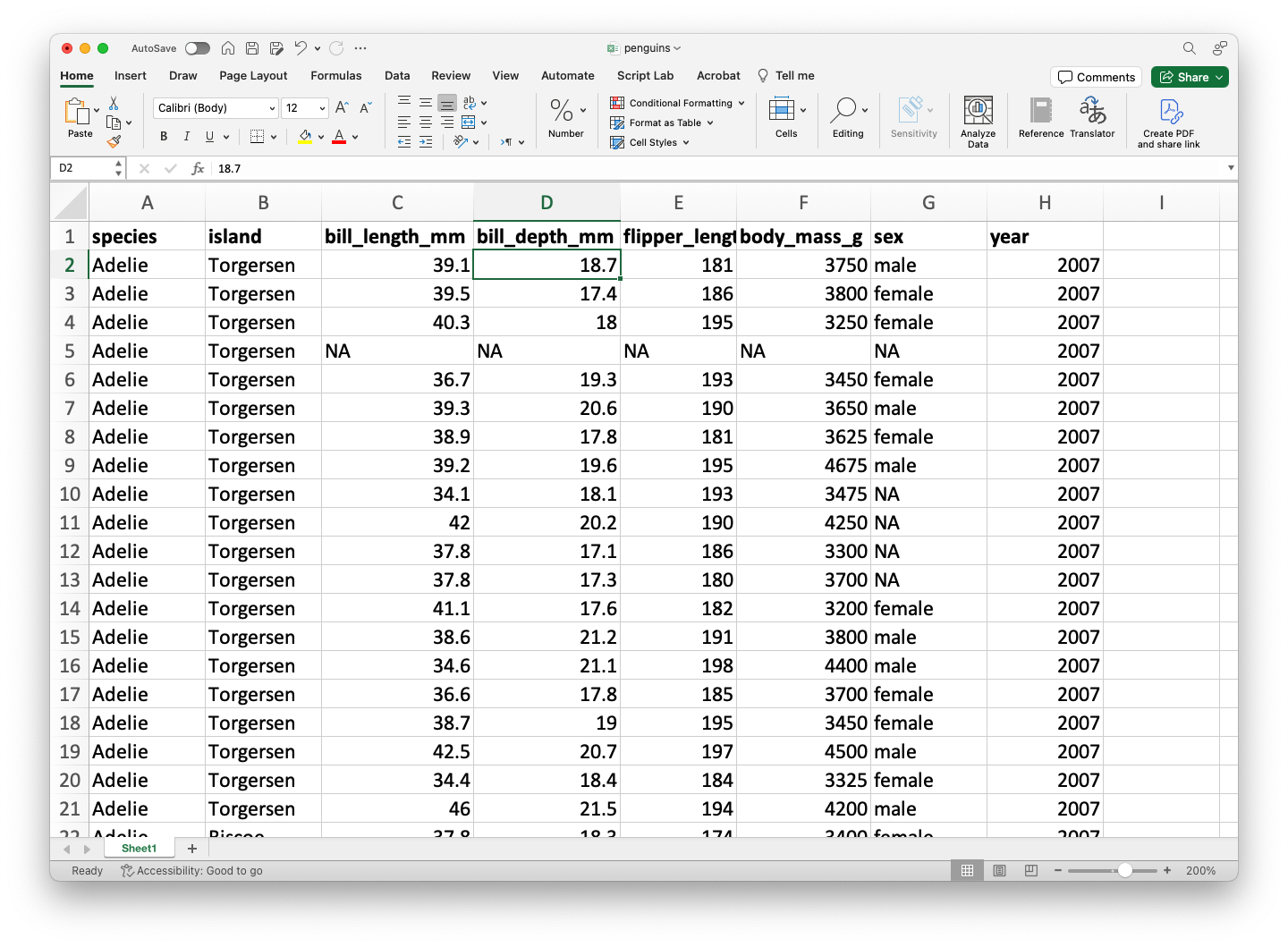

The file must be previously uploaded to Google Colab.
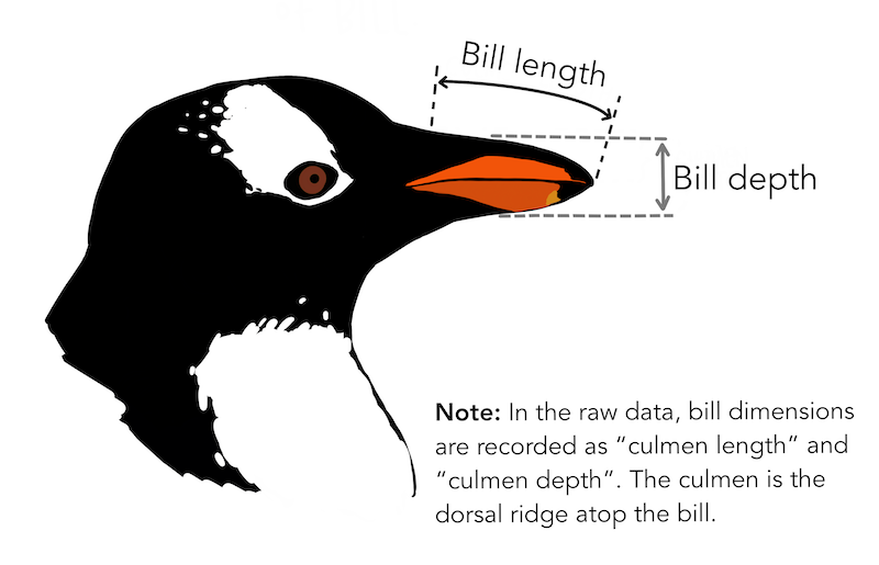
The dataset penguins.xlsx contains data from penguins living in three islands.
pandas library
![]()
- pandas is an open-source Python library for data manipulation and analysis.
- It is built on top of numpy for high-performance data operations..
- It allows the user to import, clean, transform, and analyze data efficiently
- https://pandas.pydata.org/
Importing pandas
Fortunately, the pandas library is already pre-installed in Google Colab.
However, we need to inform Google Colab that we want to use pandas and its functions using the following command:
The command as pd allows us to have a short name for pandas. To use a function of pandas, we use the command pd.function().
Loading data using pandas
The following code shows how to read the data in the file “penguins.xlsx” into Python.
The function head()
The function head() allows you to print the first rows of a pandas data frame.
| species | island | bill_length_mm | bill_depth_mm | flipper_length_mm | body_mass_g | sex | year | |
|---|---|---|---|---|---|---|---|---|
| 0 | Adelie | Torgersen | 39.1 | 18.7 | 181.0 | 3750.0 | male | 2007 |
| 1 | Adelie | Torgersen | 39.5 | 17.4 | 186.0 | 3800.0 | female | 2007 |
| 2 | Adelie | Torgersen | 40.3 | 18.0 | 195.0 | 3250.0 | female | 2007 |
| 3 | Adelie | Torgersen | NaN | NaN | NaN | NaN | NaN | 2007 |
Indexing variables a dataset
We can select a specific variables of a data frame using the syntaxis below.
0      39.1
1      39.5
2      40.3
3       NaN
4      36.7
       ...
339    55.8
340    43.5
341    49.6
342    50.8
343    50.2
Name: bill_length_mm, Length: 344, dtype: float64
Here, we selected the variable bill_length_mm in the penguins_data dataset.
To index multiple variables of a data frame, we put the names of the variables in a list object. For example, we select bill_length_mm, species, and island as follows:
Indexing rows
To index rows in a dataset, we use the argument loc from pandas. For example, we select the rows 3 to 6 of the penguins_dataset dataset:
| species | island | bill_length_mm | bill_depth_mm | flipper_length_mm | body_mass_g | sex | year | |
|---|---|---|---|---|---|---|---|---|
| 2 | Adelie | Torgersen | 40.3 | 18.0 | 195.0 | 3250.0 | female | 2007 |
| 3 | Adelie | Torgersen | NaN | NaN | NaN | NaN | NaN | 2007 |
| 4 | Adelie | Torgersen | 36.7 | 19.3 | 193.0 | 3450.0 | female | 2007 |
| 5 | Adelie | Torgersen | 39.3 | 20.6 | 190.0 | 3650.0 | male | 2007 |
Note that the index 2 and 5 refer to observations 3 and 7, respectively, in the dataset. This is because the first index in Python is 0.
Indexing rows and columns
Using loc, we can also retrieve a subset from the dataset by selecting specific columns and rows.
Return to main page
![]()
Tecnologico de Monterrey
Comments
Sometimes we write things in the coding window that we want Python to ignore. These are called comments and start with
#.Python will ignore the comments and just execute the code.