Data Manipulation and Wrangling

IN1002B: Introduction to Data Science Projects

Alan R. Vazquez

Department of Industrial Engineering

Agenda


  1. Data manipulation with pandas
  2. Basic data wrangling

Data manipulation with pandas

Chaining operations with pandas

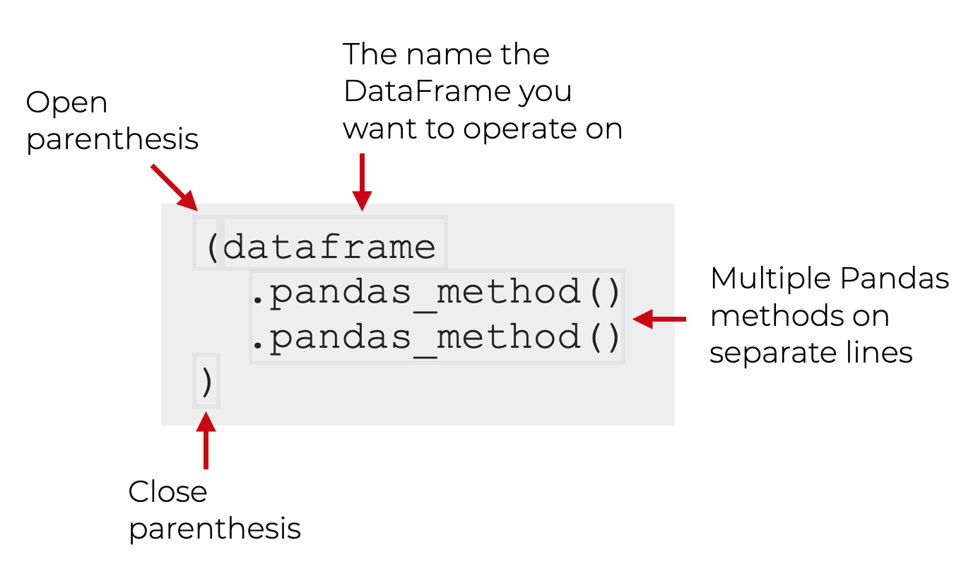
One of the most important techniques in pandas is chaining, which allows for cleaner and more readable data manipulation.

The general structure of chaining looks like this:
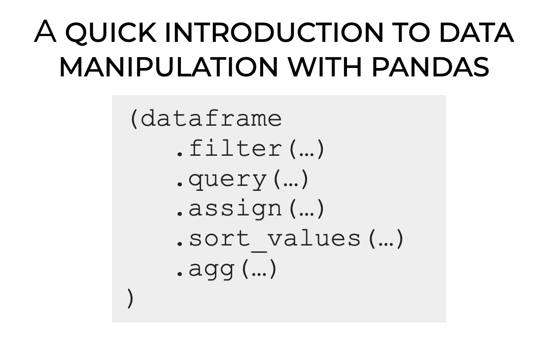
Key pandas methods

pandas provides methods or functions to solve common data manipulation tasks:

  • .filter() selects specific columns or rows.

  • .query() filters observations based on conditions.

  • .assign() adds new variables that are functions of existing variables.

  • .sort_values() changes the order of rows.

  • .agg() reduces multiple values to a single numerical summary.

To practice, we will use the dataset penguins_data.

Example 1

Let’s load the dataset and the pandas library.

import pandas as pd

# Load the Excel file into a pandas DataFrame.
penguins_data = pd.read_excel("penguins.xlsx")

# Preview the dataset.
penguins_data.head(4)
species island bill_length_mm bill_depth_mm flipper_length_mm body_mass_g sex year
0 Adelie Torgersen 39.1 18.7 181.0 3750.0 male 2007
1 Adelie Torgersen 39.5 17.4 186.0 3800.0 female 2007
2 Adelie Torgersen 40.3 18.0 195.0 3250.0 female 2007
3 Adelie Torgersen NaN NaN NaN NaN NaN 2007

Selecting columns with .filter()

Select the columns species, body_mass_g and sex.

(penguins_data
  .filter(["species", "body_mass_g", "sex"], axis = 1)
).head()
species body_mass_g sex
0 Adelie 3750.0 male
1 Adelie 3800.0 female
2 Adelie 3250.0 female
3 Adelie NaN NaN
4 Adelie 3450.0 female


The axis argument tells .filter() whether to select rows (0) or columns (1) from the dataframe.

(penguins_data
  .filter(["species", "body_mass_g", "sex"], axis = 1)
).head()


The .head() command allows us to print the first six rows of the newly produced dataframe. We must remove it to have the entire new dataframe.


We can also use .filter() to select rows too. To this end, we set axis = 1. We can select specific rows, such as 0 and 10.

(penguins_data
  .filter([0, 10], axis = 0)
)
species island bill_length_mm bill_depth_mm flipper_length_mm body_mass_g sex year
0 Adelie Torgersen 39.1 18.7 181.0 3750.0 male 2007
10 Adelie Torgersen 37.8 17.1 186.0 3300.0 NaN 2007

Or, we can select a set of rows using the function range(). For example, let’s select the first 5 rows.

(penguins_data
  .filter(range(5), axis = 0)
)
species island bill_length_mm bill_depth_mm flipper_length_mm body_mass_g sex year
0 Adelie Torgersen 39.1 18.7 181.0 3750.0 male 2007
1 Adelie Torgersen 39.5 17.4 186.0 3800.0 female 2007
2 Adelie Torgersen 40.3 18.0 195.0 3250.0 female 2007
3 Adelie Torgersen NaN NaN NaN NaN NaN 2007
4 Adelie Torgersen 36.7 19.3 193.0 3450.0 female 2007

Filtering rows with .query()


An alternative way of selecting rows is .query(). Compared to .filter(), .query() allows us to filter the data using statements or queries involving the variables.


For example, let’s filter the data for the species “Gentoo.”

(penguins_data
  .query("species == 'Gentoo'")
)


(penguins_data
  .query("species == 'Gentoo'")
).head()
species island bill_length_mm bill_depth_mm flipper_length_mm body_mass_g sex year
152 Gentoo Biscoe 46.1 13.2 211.0 4500.0 female 2007
153 Gentoo Biscoe 50.0 16.3 230.0 5700.0 male 2007
154 Gentoo Biscoe 48.7 14.1 210.0 4450.0 female 2007
155 Gentoo Biscoe 50.0 15.2 218.0 5700.0 male 2007
156 Gentoo Biscoe 47.6 14.5 215.0 5400.0 male 2007

We can also filter the data to get penguins with a body mass greater than 5000g.

(penguins_data
  .query("body_mass_g > 5000")
).head()
species island bill_length_mm bill_depth_mm flipper_length_mm body_mass_g sex year
153 Gentoo Biscoe 50.0 16.3 230.0 5700.0 male 2007
155 Gentoo Biscoe 50.0 15.2 218.0 5700.0 male 2007
156 Gentoo Biscoe 47.6 14.5 215.0 5400.0 male 2007
159 Gentoo Biscoe 46.7 15.3 219.0 5200.0 male 2007
161 Gentoo Biscoe 46.8 15.4 215.0 5150.0 male 2007

We can even combine .filter() and .query(). For example, let’s select the columns species, body_mass_g and sex, then filter the data for the “Gentoo” species.

(penguins_data
  .filter(["species", "body_mass_g", "sex"], axis = 1)
  .query("species == 'Gentoo'")
).head(4)
species body_mass_g sex
152 Gentoo 4500.0 female
153 Gentoo 5700.0 male
154 Gentoo 4450.0 female
155 Gentoo 5700.0 male

Create new columns with .assign()

With .assign(), we can create new columns (variables) that are functions of existing ones. This function uses a special Python keyword called lambda. Technically, this keyword defines an anonymous function.

For example, we create a new variable LDRatio equaling the ratio of bill_length_mm and bill_depth_mm.

(penguins_data
  .assign(LDRatio = lambda df: df["bill_length_mm"] / df["bill_depth_mm"])
)


In this code, the df after lambda indicates that the dataframe (penguins_data) will be referred to as df inside the function. The colon : sets the start of the function.

(penguins_data
  .assign(LDRatio = lambda df: df["bill_length_mm"] / df["bill_depth_mm"])
)

The code appends the new variable to the end of the resulting dataframe.

We can see the new variable using .filter().

(penguins_data
  .assign(LDRatio = lambda df: df["bill_length_mm"] / df["bill_depth_mm"])
  .filter(["bill_length_mm", "bill_depth_mm", "LDRatio"], axis = 1)
).head()
bill_length_mm bill_depth_mm LDRatio
0 39.1 18.7 2.090909
1 39.5 17.4 2.270115
2 40.3 18.0 2.238889
3 NaN NaN NaN
4 36.7 19.3 1.901554

Sorting with .sort_values()

We can sort the data based on a column like bill_length_mm.

(penguins_data
  .sort_values("bill_length_mm")
).head(4)
species island bill_length_mm bill_depth_mm flipper_length_mm body_mass_g sex year
142 Adelie Dream 32.1 15.5 188.0 3050.0 female 2009
98 Adelie Dream 33.1 16.1 178.0 2900.0 female 2008
70 Adelie Torgersen 33.5 19.0 190.0 3600.0 female 2008
92 Adelie Dream 34.0 17.1 185.0 3400.0 female 2008

To sort in descending order, use ascending=False inside sort_values().

(penguins_data
  .sort_values("bill_length_mm", ascending=False)
).head()
species island bill_length_mm bill_depth_mm flipper_length_mm body_mass_g sex year
185 Gentoo Biscoe 59.6 17.0 230.0 6050.0 male 2007
293 Chinstrap Dream 58.0 17.8 181.0 3700.0 female 2007
253 Gentoo Biscoe 55.9 17.0 228.0 5600.0 male 2009
339 Chinstrap Dream 55.8 19.8 207.0 4000.0 male 2009
267 Gentoo Biscoe 55.1 16.0 230.0 5850.0 male 2009

Summarizing with .agg()

We can calculate summary statistics of the columns bill_length_mm, bill_depth_mm, and body_mass_g.

(penguins_data
  .filter(["bill_length_mm", "bill_depth_mm", "body_mass_g"], axis = 1)
  .agg(["mean"])
)
bill_length_mm bill_depth_mm body_mass_g
mean 43.92193 17.15117 4201.754386


By default, agg() ignores missing values.

Saving results in new objects


After performing operations on our data, we can save the modified dataset as a new object.

mean_penguins_data = (penguins_data
  .filter(["bill_length_mm", "bill_depth_mm", "body_mass_g"], axis = 1)
  .agg(["mean"])
)

mean_penguins_data
bill_length_mm bill_depth_mm body_mass_g
mean 43.92193 17.15117 4201.754386

More on pandas

https://wesmckinney.com/book/

Basic data wrangling

Data wrangling


  • Data wrangling is the process of transforming raw data into a clean and structured format.

  • It involves merging, reshaping, filtering, and organizing data for analysis.

  • Here, we illustrate some special functions of the pandas for cleaning common issues with a dataset.

Example 2

Consider an industrial engineer who receives a messy Excel file from a manufacturing client. The data file is called “industrial_dataset.xlsx”, which file includes data about machine maintenance logs, production output, and operator comments.

The goal is to clean and prepare this dataset using pandas so it can be analyzed.

Let’s read the data set into Python.

# Load the Excel file into a pandas DataFrame.
client_data = pd.read_excel("industrial_dataset.xlsx")

# Preview the dataset.
client_data.head()
Machine ID Output (units) Maintenance Date Operator Comment
0 101 1200 2023-01-10 Ana ok
1 101 1200 2023-01-10 Ana ok
2 102 1050 2023-01-12 Bob Needs oil!
3 103 error 2023-01-13 Charlie All good\n
4 103 950 2023-01-13 Charlie All good\n

Remove duplicate rows


Duplicate or identical rows are rows that have the same entries in every column in the dataset.

If only one row is needed for the analysis, we can remove the duplicates using the .drop_duplicates() function.

client_data_single = (client_data
                     .drop_duplicates()
                      )

The client_data_single dataframe does not have duplicate rows.

client_data_single.head()
Machine ID Output (units) Maintenance Date Operator Comment
0 101 1200 2023-01-10 Ana ok
1 101 1200 2023-01-10 Ana ok
2 102 1050 2023-01-12 Bob Needs oil!
3 103 error 2023-01-13 Charlie All good\n
4 103 950 2023-01-13 Charlie All good\n

Add an index column


In some cases, it is useful to have a unique identifier for each row in the dataset. We can create an identifier using the function .assign with some extra syntaxis.

client_data_single = (client_data_single
                      .reset_index(drop = True)
                      .assign(ID = lambda x: x.index + 1)
                      ) 

The new column is appended to the end of the dataframe.

client_data_single.head()
Machine ID Output (units) Maintenance Date Operator Comment ID
0 101 1200 2023-01-10 Ana ok 1
1 101 1200 2023-01-10 Ana ok 2
2 102 1050 2023-01-12 Bob Needs oil! 3
3 103 error 2023-01-13 Charlie All good\n 4
4 103 950 2023-01-13 Charlie All good\n 5

To bring it to the begining of the array, we can use the .filter() function.

client_data_single = (client_data_single
.filter(['ID', 'Machine ID',    'Output (units)',   
        'Maintenance Date', 'Operator', 'Comment'])
)
client_data_single.head(3)  
ID Machine ID Output (units) Maintenance Date Operator Comment
0 1 101 1200 2023-01-10 Ana ok
1 2 101 1200 2023-01-10 Ana ok
2 3 102 1050 2023-01-12 Bob Needs oil!

Fill blank cells

In the dataset, there are columns with missing values. If we would like to fill them with specific values or text, we use the .fillna() function. In this function, we use the syntaxis 'Variable': 'Replace', where the Variable is the column in the dataset and Replace is the text or number to fill the entry in.

Let’s fill in the missing entries of the columns Operator, Maintenance Date, and Comment.

complete_data = (client_data_single
                .fillna({'Operator': 'Unknown', 
                'Maintenance Date': '2023-01-01',
                'Comment': 'None'})
                ) 

complete_data.head()
ID Machine ID Output (units) Maintenance Date Operator Comment
0 1 101 1200 2023-01-10 Ana ok
1 2 101 1200 2023-01-10 Ana ok
2 3 102 1050 2023-01-12 Bob Needs oil!
3 4 103 error 2023-01-13 Charlie All good\n
4 5 103 950 2023-01-13 Charlie All good\n

Replace values


There are some cases in which columns have some undesired or unwatned values. Consider the Output (units) as an example.

complete_data['Output (units)'].head()
0     1200
1     1200
2     1050
3    error
4      950
Name: Output (units), dtype: object

The column has the numbers of units but also text such as “error”.


We can replace the “error” in this column by a user-specified value, say, 0. To this end, we use the function .replace(). The function has two inputs. The first one is the value to replace and the second one is the replacement value.

complete_data['Output (units)'] = complete_data['Output (units)'].replace('error', 0)


Let’s check the new column.

complete_data['Output (units)']
0     1200
1     1200
2     1050
3        0
4      950
      ... 
95     800
96    1100
97     950
98     950
99    1100
Name: Output (units), Length: 100, dtype: int64

Note that the new column is now numeric.

Split column into multiple ones

There are some cases in which we want to split a column according to a character. For example, consider the column Comment from the dataset.

complete_data['Comment']
0                       ok
1                       ok
2               Needs oil!
3               All good\n
4               All good\n
              ...         
95    Requires part: valve
96                      ok
97    Delay: maintenance\n
98              Needs oil!
99              All good\n
Name: Comment, Length: 100, dtype: object

The column has some values such as “Requires part: valve” and “Delay: maintenance” that we may want to split into columns.

0                       ok
1                       ok
2               Needs oil!
3               All good\n
4               All good\n
              ...         
95    Requires part: valve
96                      ok
97    Delay: maintenance\n
98              Needs oil!
99              All good\n
Name: Comment, Length: 100, dtype: object


We can split the values in the column according to the colon “:”.

That is, everything before the colon will be in a column. Everything after the colon will be in another column. To achieve this, we use the function str.split().

One input of the function is the symbol or character for which we cant to make a split. The other input, expand = True tells Python that we want to create new columns.

complete_data['Comment'].str.split(':', expand = True)

The result is two columns.

split_column = complete_data['Comment'].str.split(':', expand = True)
split_column.head()
0 1
0 ok None
1 ok None
2 Needs oil! None
3 All good\n None
4 All good\n None


We can assign them to new columns in the dataset using the following code.

augmented_data = (complete_data
                  .assign(First_comment = split_column.filter([0]),
                  Second_comment = split_column.filter([1]))
                  )

augmented_data.head()
ID Machine ID Output (units) Maintenance Date Operator Comment First_comment Second_comment
0 1 101 1200 2023-01-10 Ana ok ok None
1 2 101 1200 2023-01-10 Ana ok ok None
2 3 102 1050 2023-01-12 Bob Needs oil! Needs oil! None
3 4 103 0 2023-01-13 Charlie All good\n All good\n None
4 5 103 950 2023-01-13 Charlie All good\n All good\n None

Remove characters


Something that we notice is that the column First_Comment has some extra characters like “” that may be useless when working with the data.

We can remove them using the function str.strip(). The input of the function is the character to remove.

augmented_data['First_comment'] = augmented_data['First_comment'].str.strip("\n")


Let’s see the cleaned column.

augmented_data['First_comment']
0                ok
1                ok
2        Needs oil!
3          All good
4          All good
          ...      
95    Requires part
96               ok
97            Delay
98       Needs oil!
99         All good
Name: First_comment, Length: 100, dtype: object


We can also remove other characters.

augmented_data['First_comment'].str.strip("!")
0                ok
1                ok
2         Needs oil
3          All good
4          All good
          ...      
95    Requires part
96               ok
97            Delay
98        Needs oil
99         All good
Name: First_comment, Length: 100, dtype: object

Transform text case

When working with text columns such as those containing names, it might be possible to have different ways of writing. A common case is when having lower case or upper case names or a combination thereof.

For example, consider the column Operator containing the names of the operators.

complete_data['Operator'].head()
0       Ana 
1        Ana
2        Bob
3    Charlie
4    Charlie
Name: Operator, dtype: object

Remove extra spaces


To deal with names, we first use the .str.strip() to remove leading and trailing characters from strings.

complete_data['Operator'] = complete_data['Operator'].str.strip()
complete_data['Operator']
0         Ana
1         Ana
2         Bob
3     Charlie
4     Charlie
       ...   
95    Charlie
96        Ana
97        Ana
98    Charlie
99        ana
Name: Operator, Length: 100, dtype: object

Change to lowercase letters


We can turn all names to lowercase using the function str.lower().

complete_data['Operator'].str.lower()
0         ana
1         ana
2         bob
3     charlie
4     charlie
       ...   
95    charlie
96        ana
97        ana
98    charlie
99        ana
Name: Operator, Length: 100, dtype: object

Change to uppercase letters


We can turn all names to lowercase using the function str.upper().

complete_data['Operator'].str.upper()
0         ANA
1         ANA
2         BOB
3     CHARLIE
4     CHARLIE
       ...   
95    CHARLIE
96        ANA
97        ANA
98    CHARLIE
99        ANA
Name: Operator, Length: 100, dtype: object

Capitalize the first letter


We can convert all names to title case using the function str.title().

complete_data['Operator'].str.title()
0         Ana
1         Ana
2         Bob
3     Charlie
4     Charlie
       ...   
95    Charlie
96        Ana
97        Ana
98    Charlie
99        Ana
Name: Operator, Length: 100, dtype: object

Return to main page