Classification Trees

IN2004B: Generation of Value with Data Analytics

Alan R. Vazquez

Department of Industrial Engineering

Agenda

1. Introduction
2. Training, Validation, and Test Data
3. Classification Trees
4. Classification Algorithm Metrics

Introduction

Load the libraries

Before we start, let’s import the data science libraries into Python.

import pandas as pd
import matplotlib.pyplot as plt
import seaborn as sns
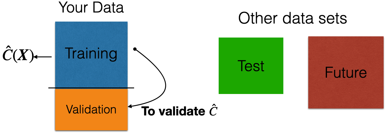
from sklearn.model_selection import train_test_split
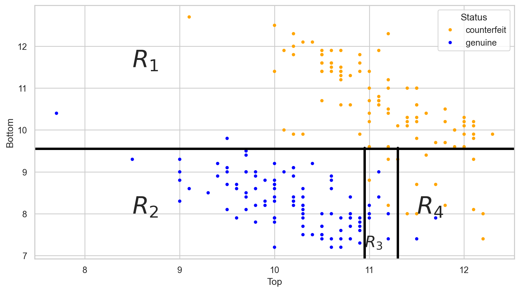
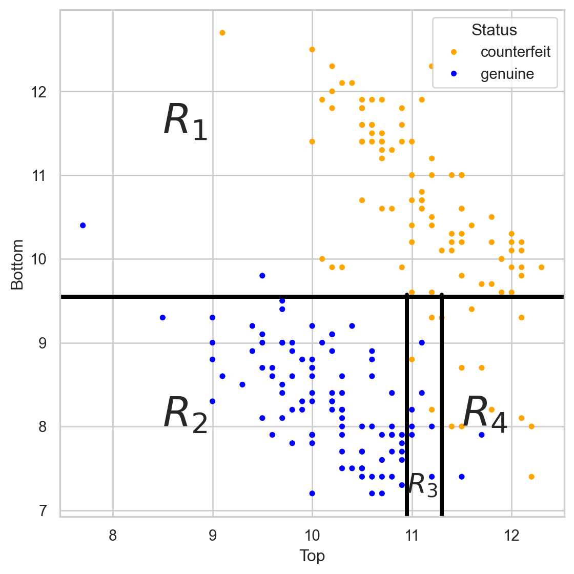
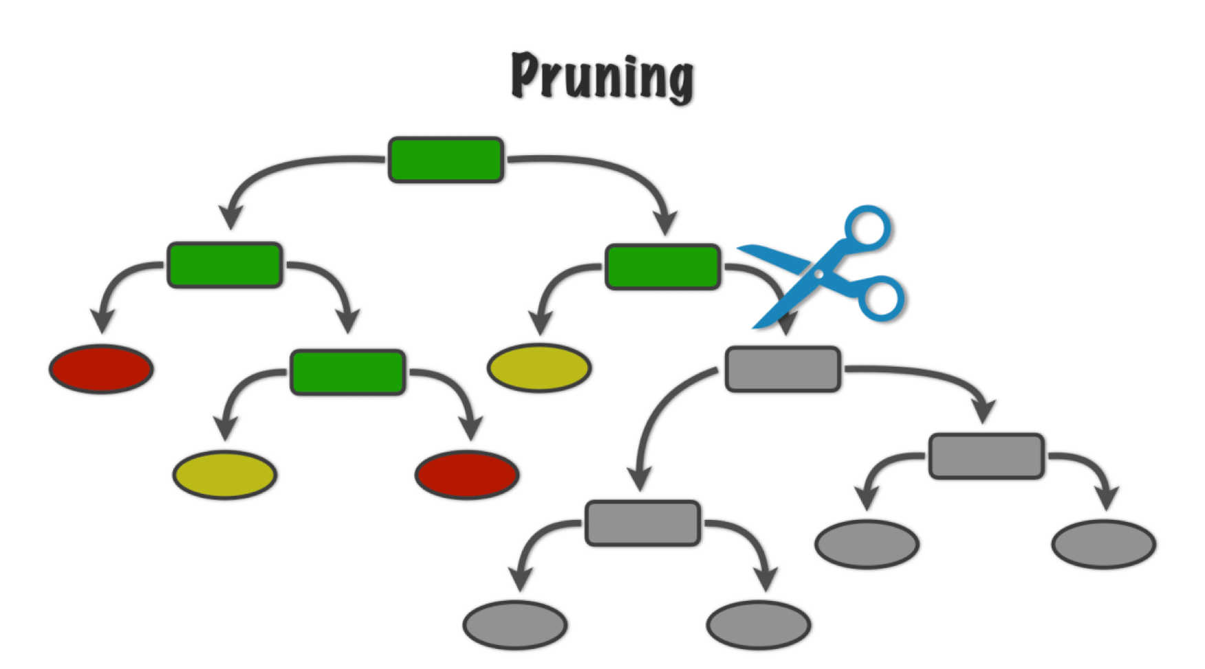
from sklearn.tree import DecisionTreeClassifier, plot_tree
from sklearn.preprocessing import StandardScaler
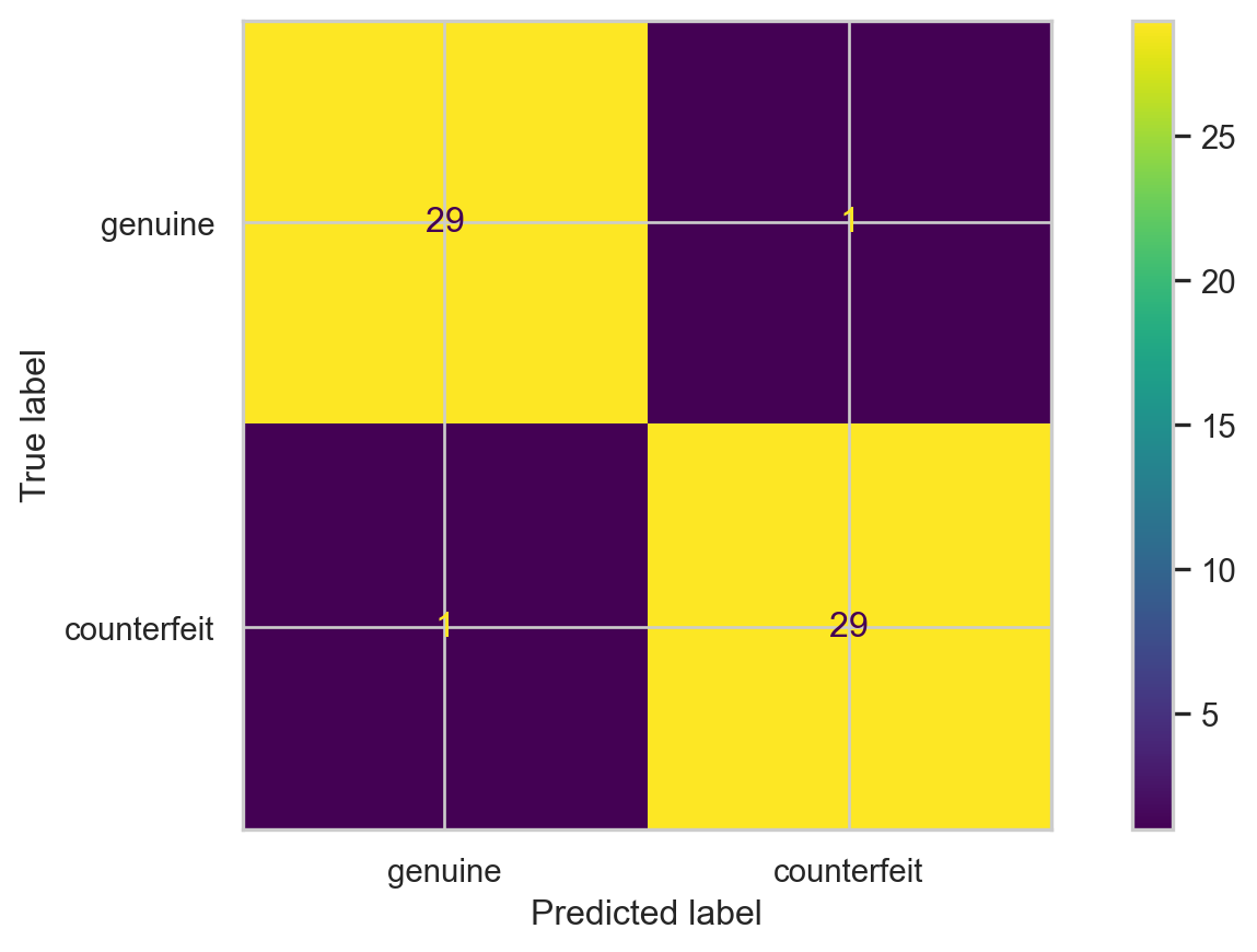
from sklearn.metrics import confusion_matrix, ConfusionMatrixDisplay 
from sklearn.metrics import accuracy_score, recall_score, precision_score

Here, we use specific functions from the pandas, matplotlib, seaborn and sklearn libraries in Python.

scikit-learn library

• scikit-learn is a robust and popular library for machine learning in Python
• It provides simple, efficient tools for data mining and data analysis
• It is built on top of libraries such as NumPy, SciPy, and Matplotlib
• https://scikit-learn.org/stable/

Main data science problems

Regression Problems. The response is numerical. For example, a person’s income, the value of a house, or a patient’s blood pressure.

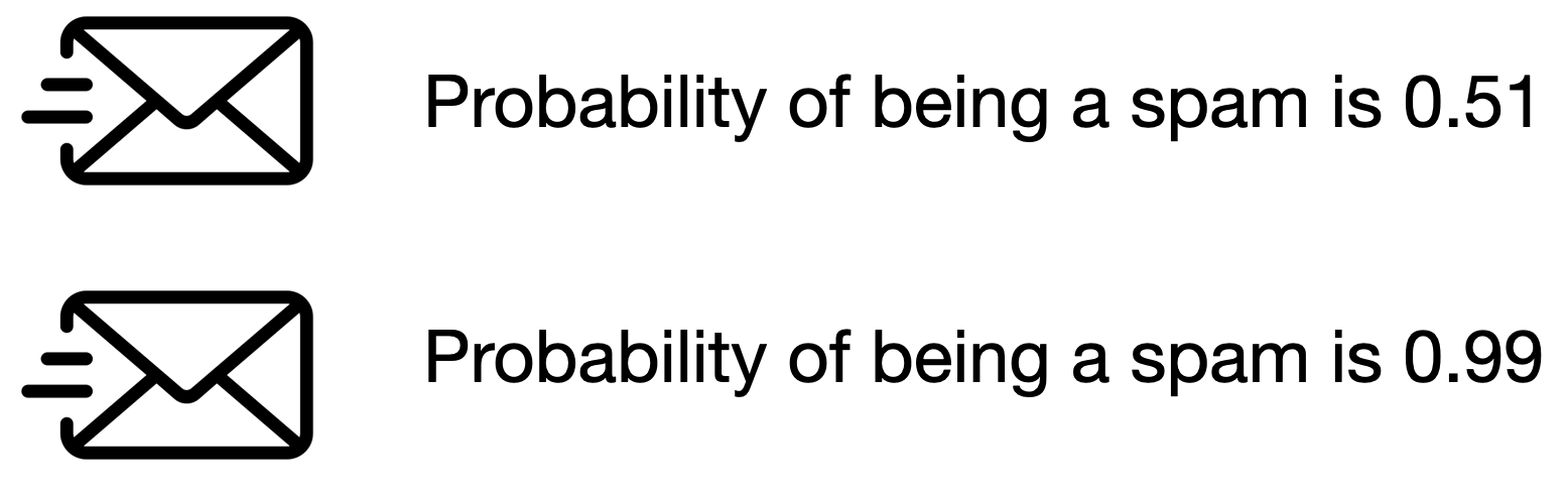
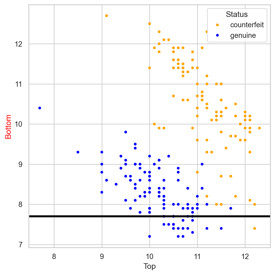
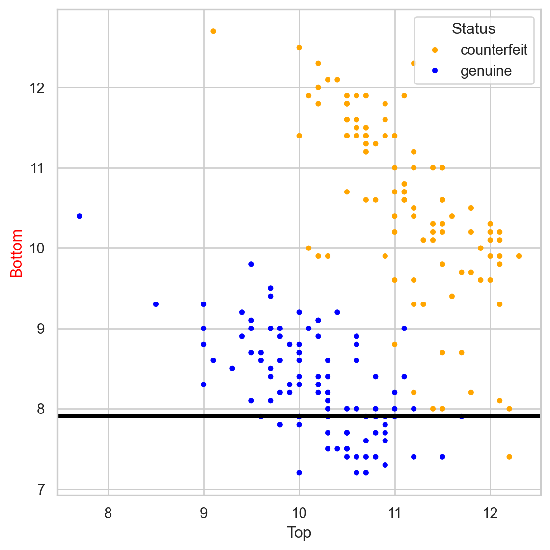
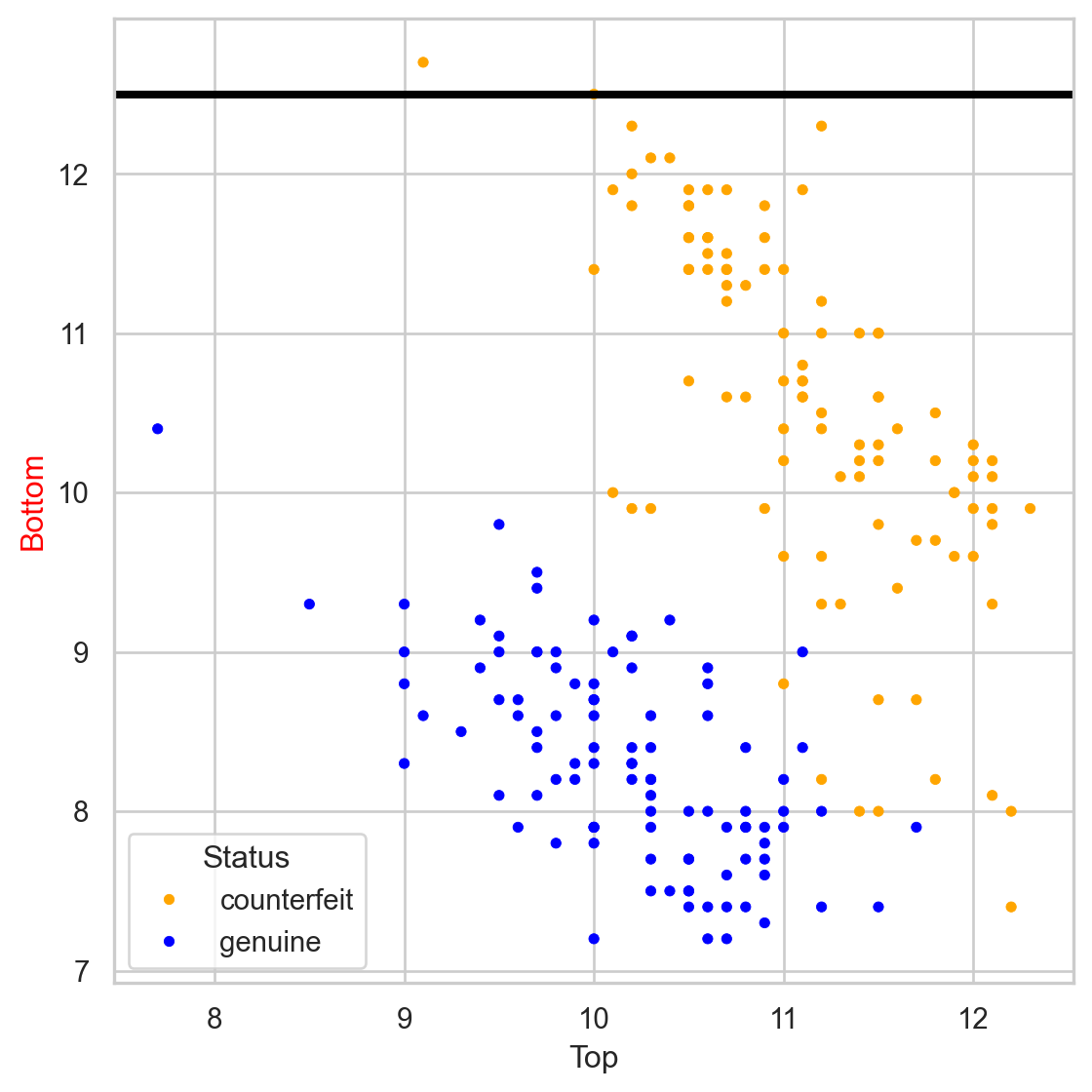
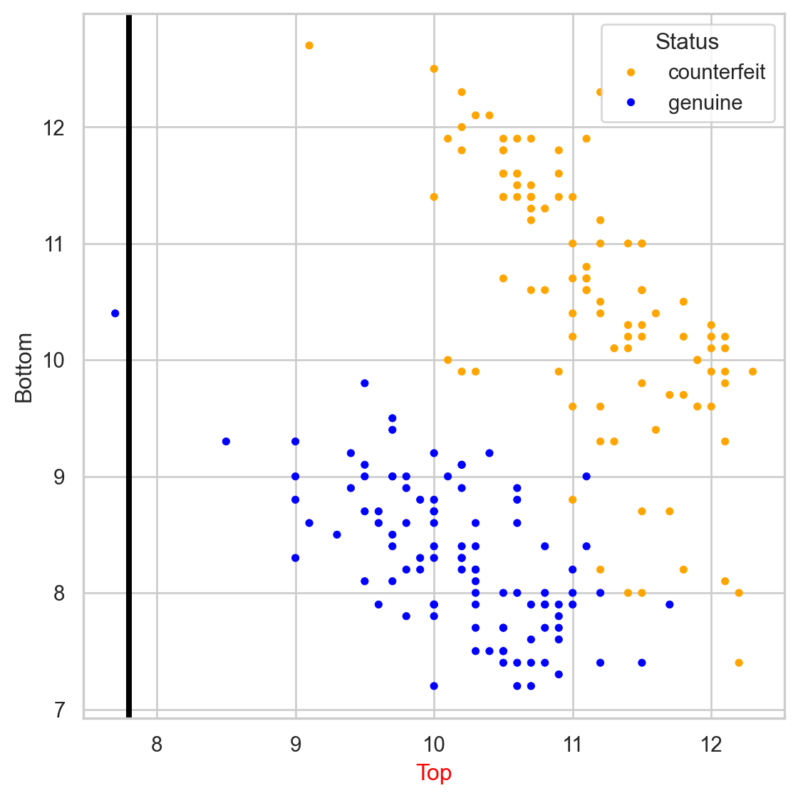
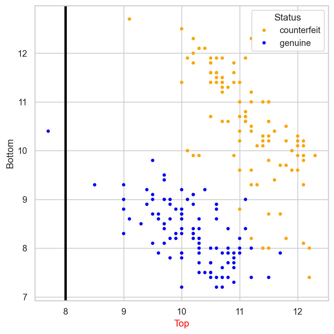
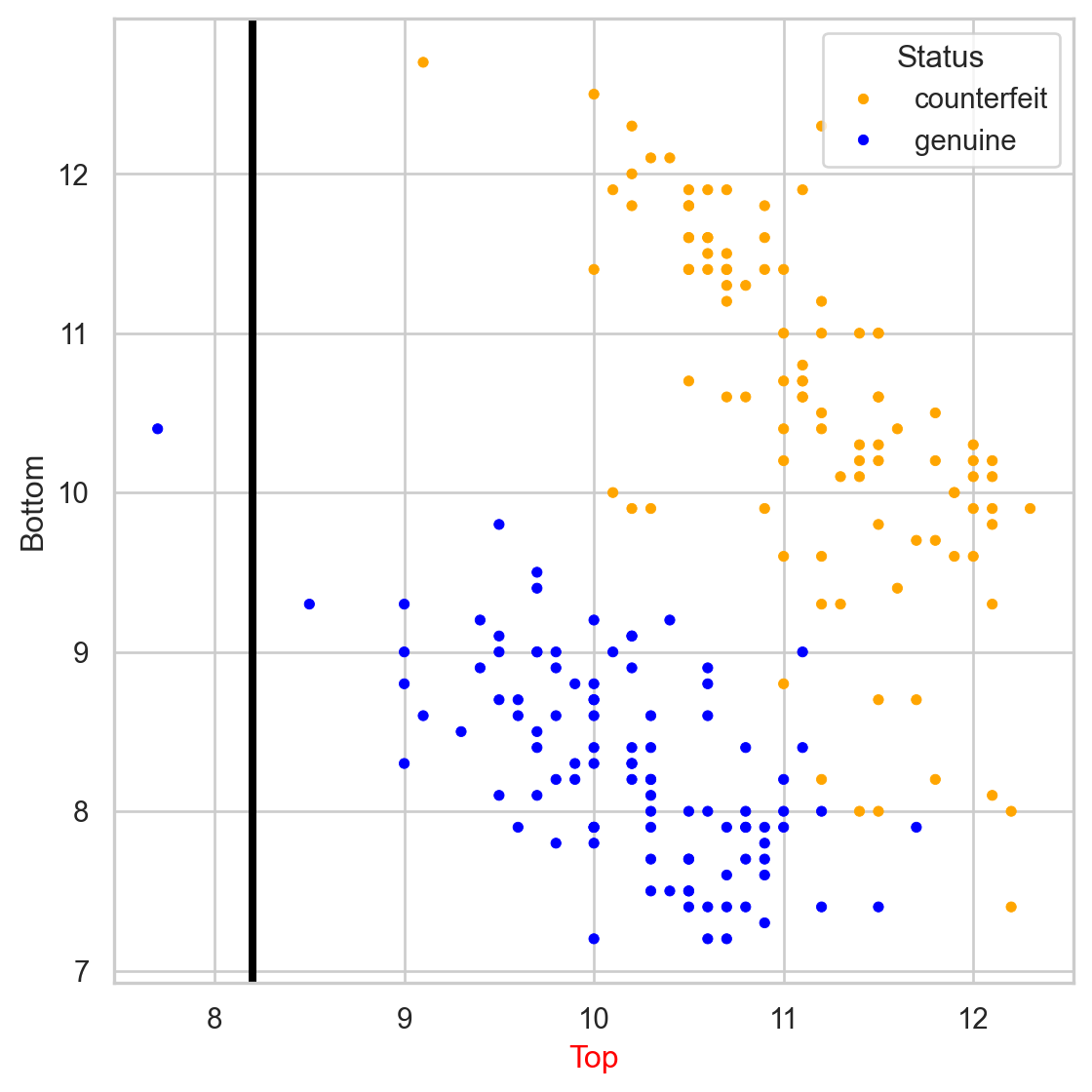
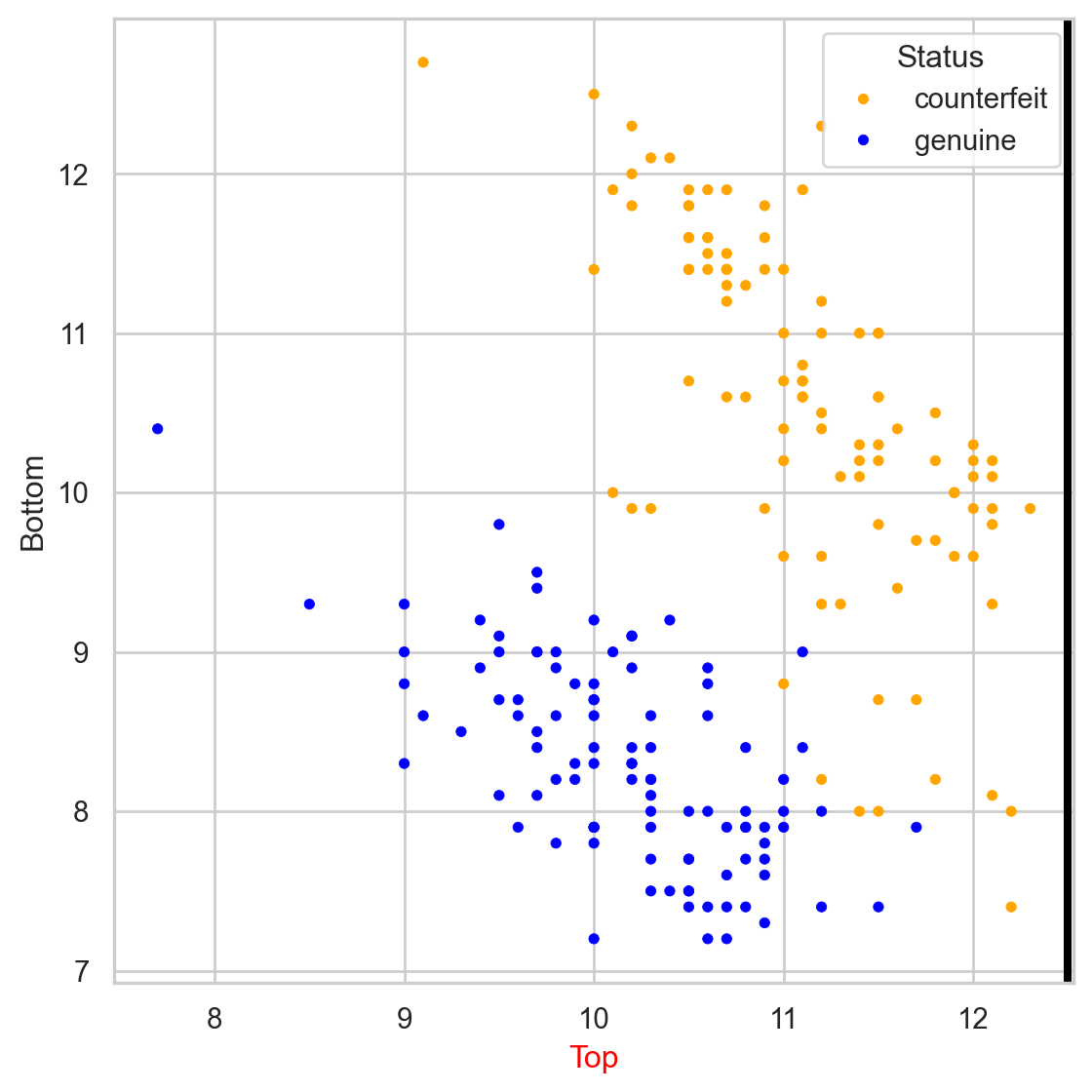
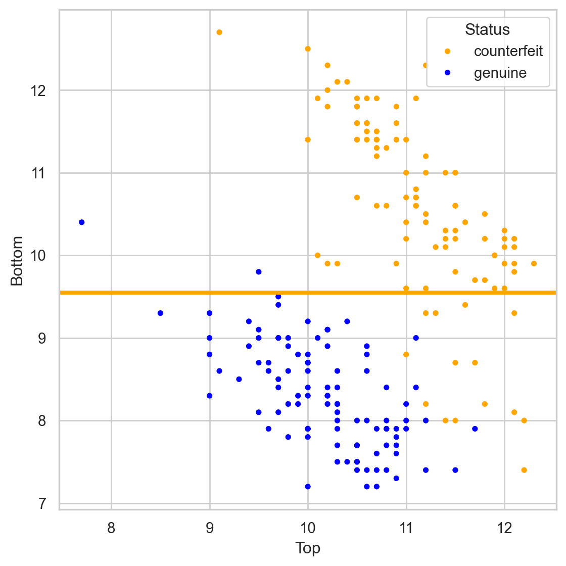
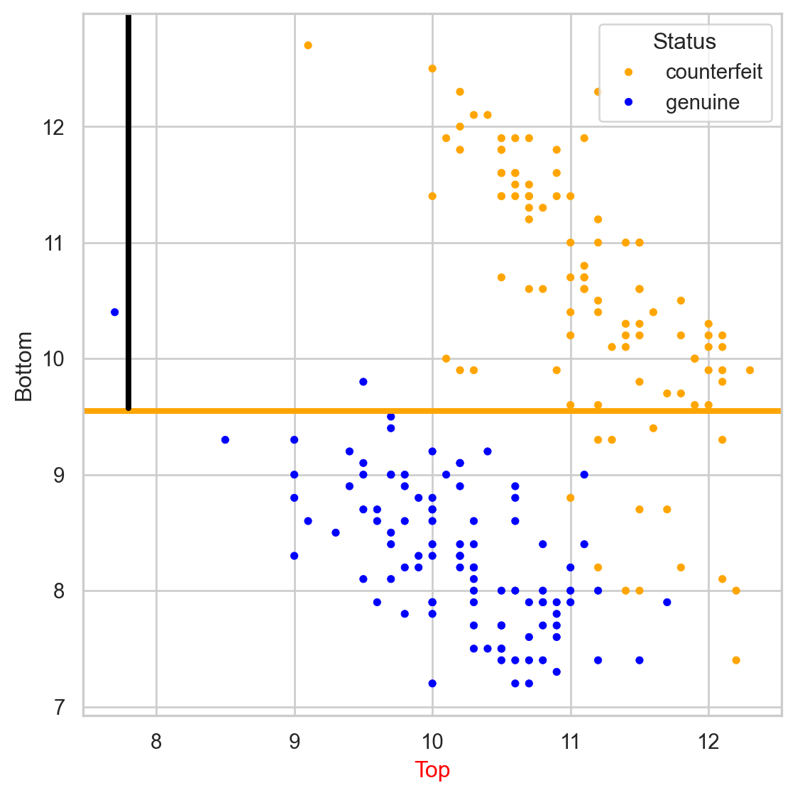
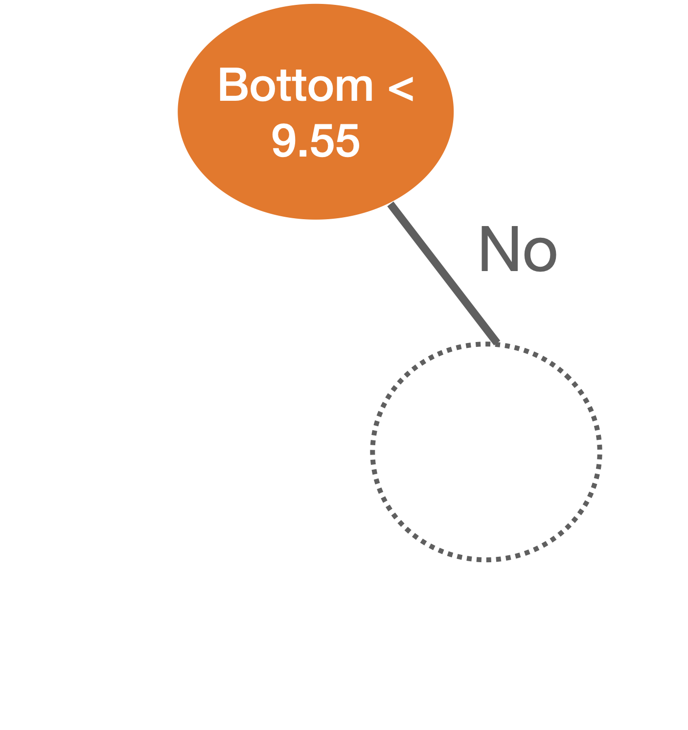
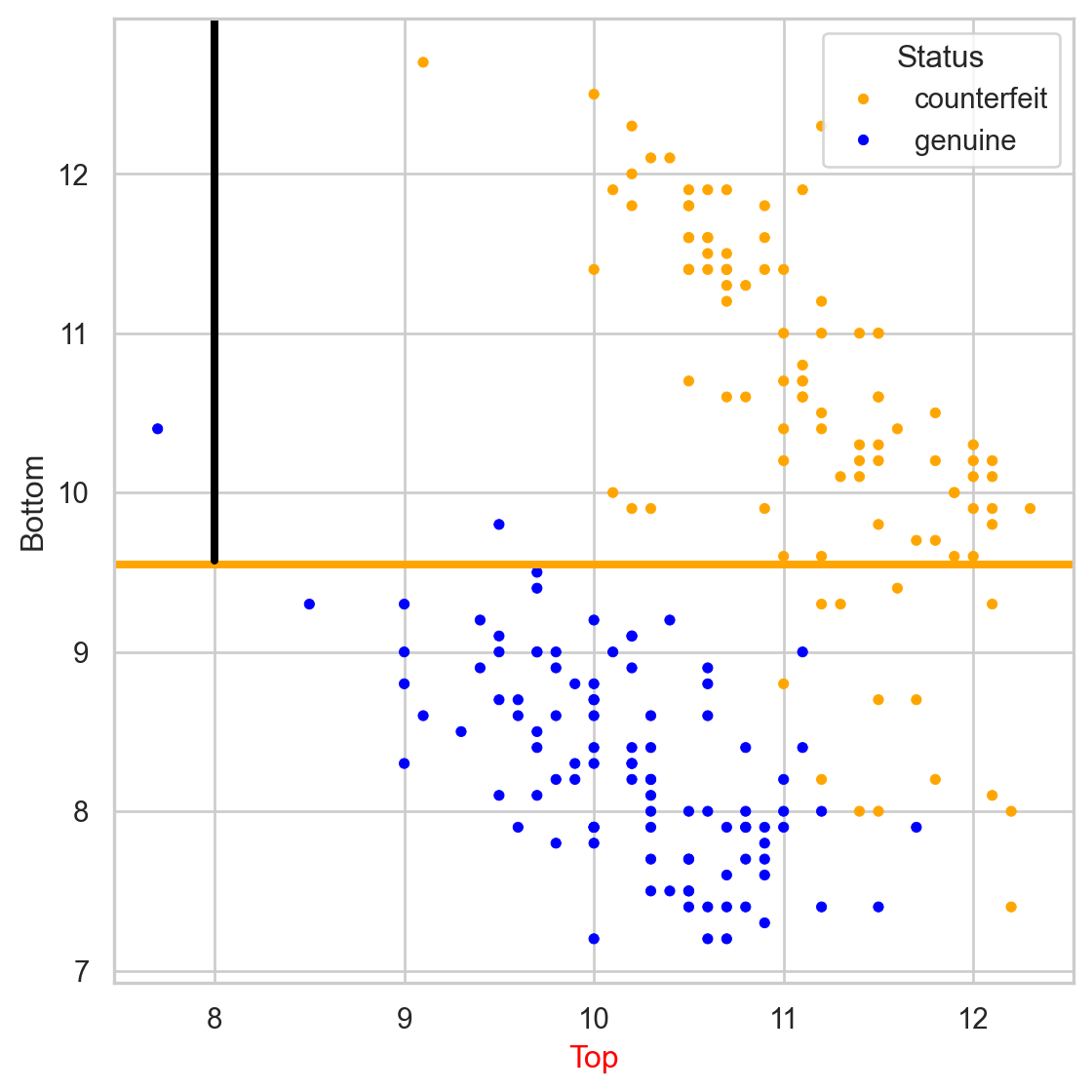
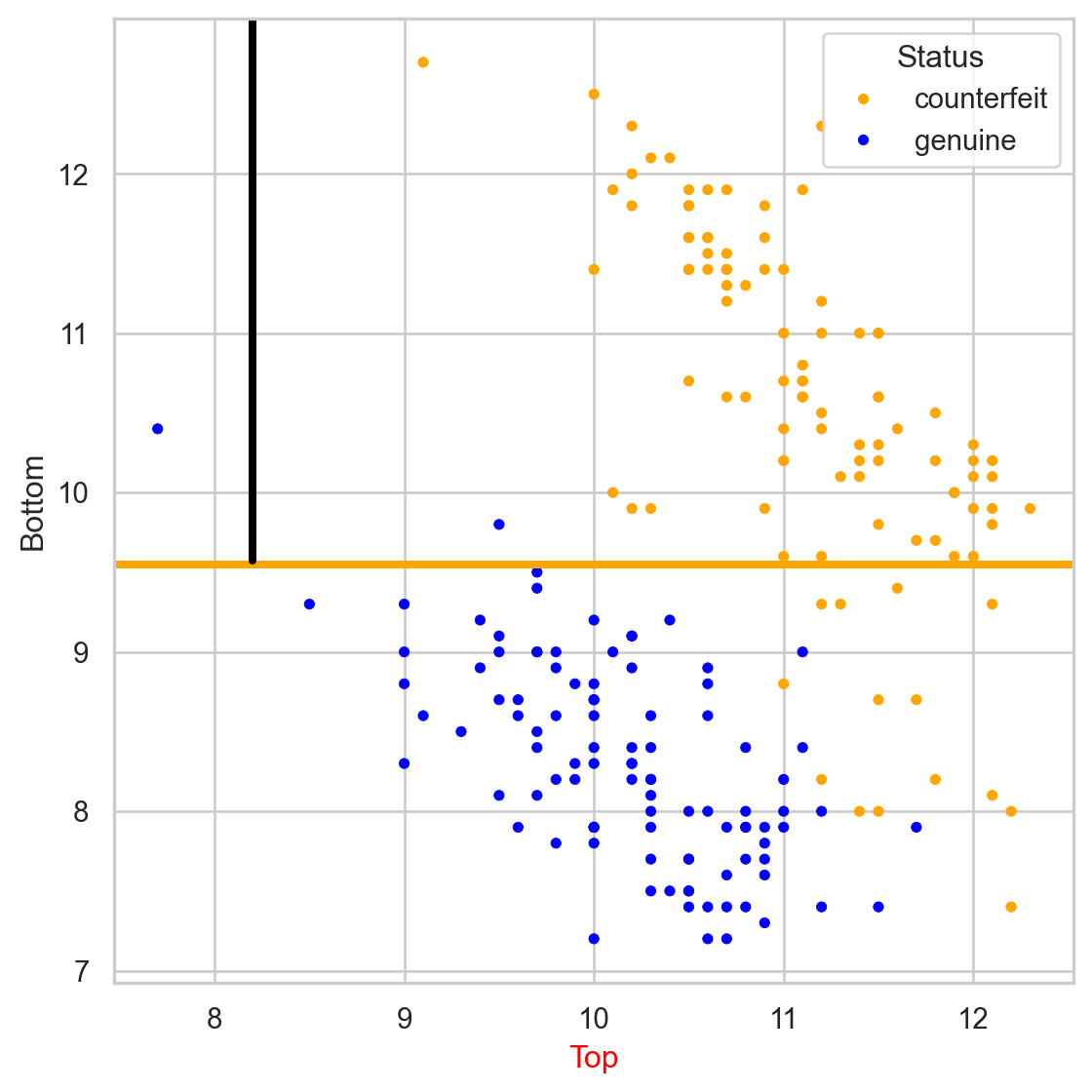
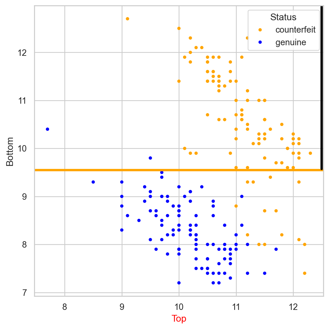
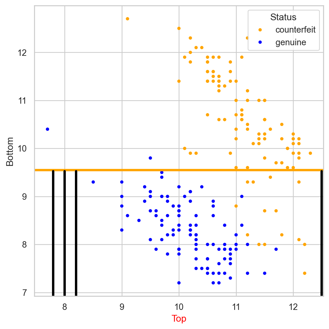
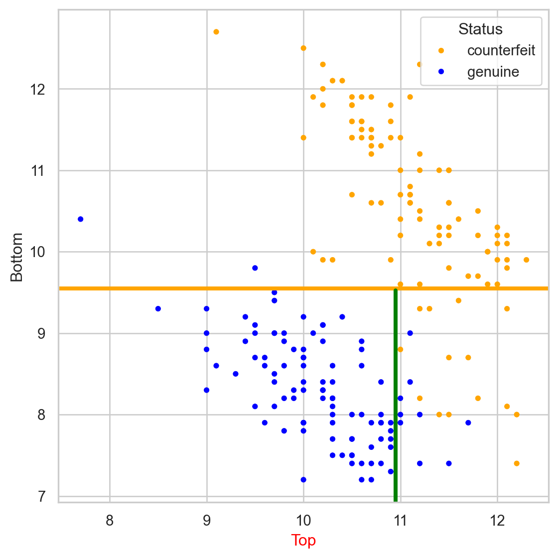
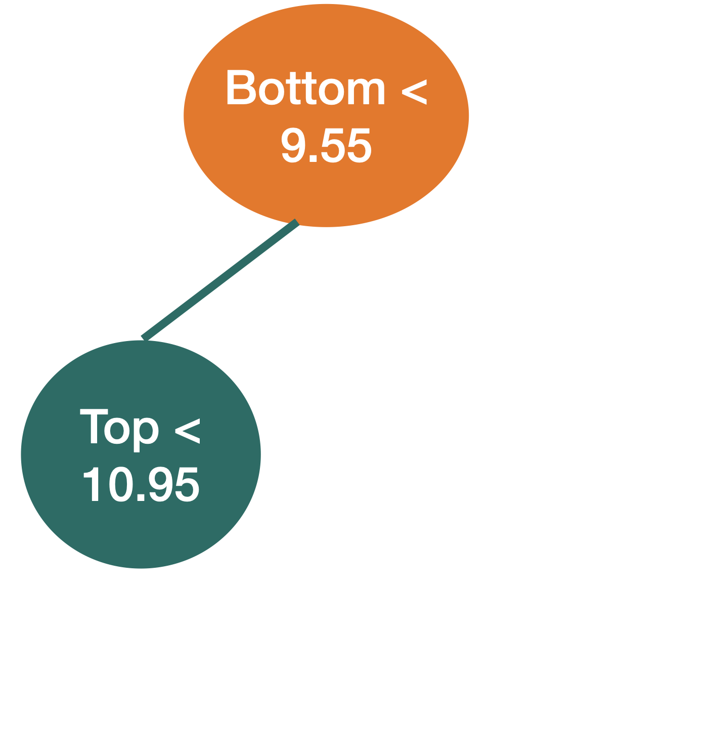
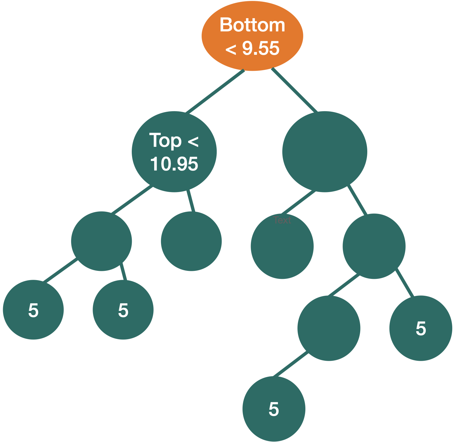
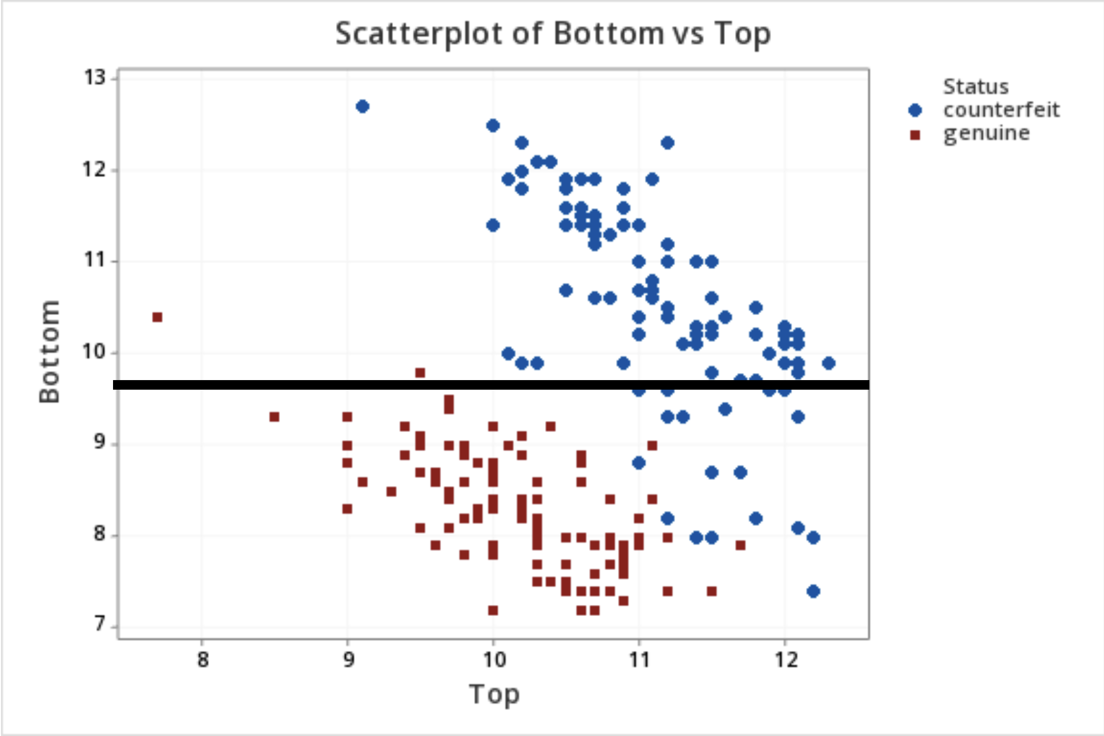
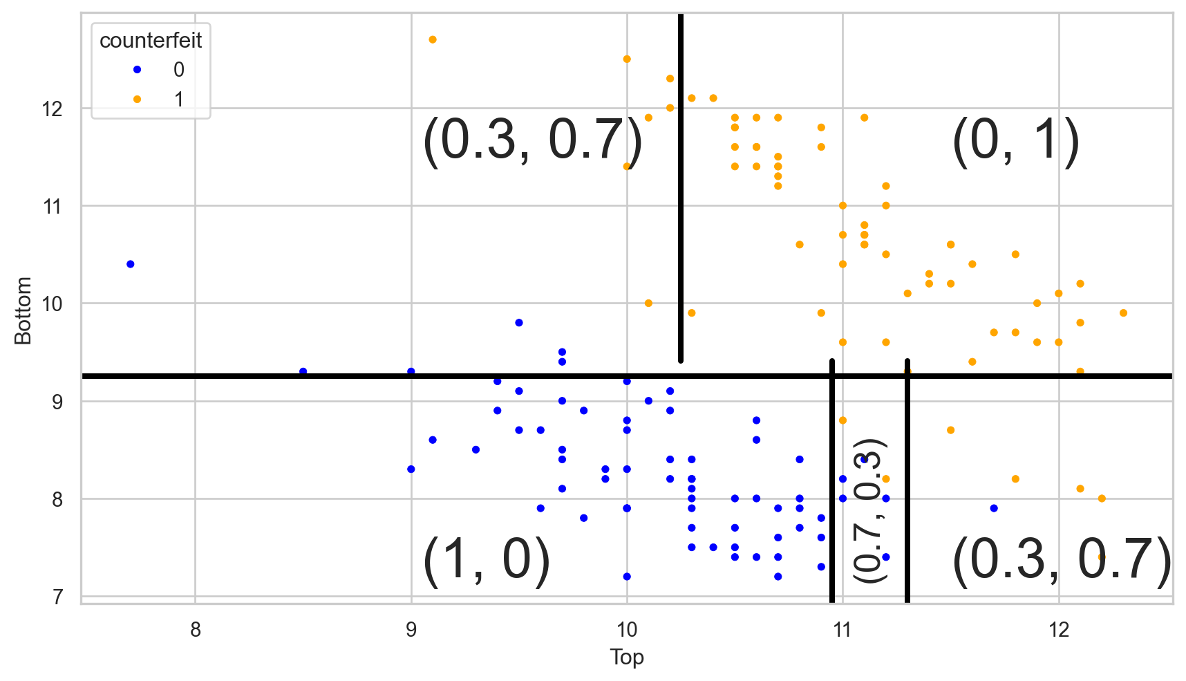
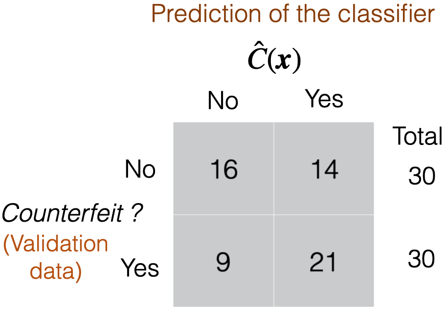
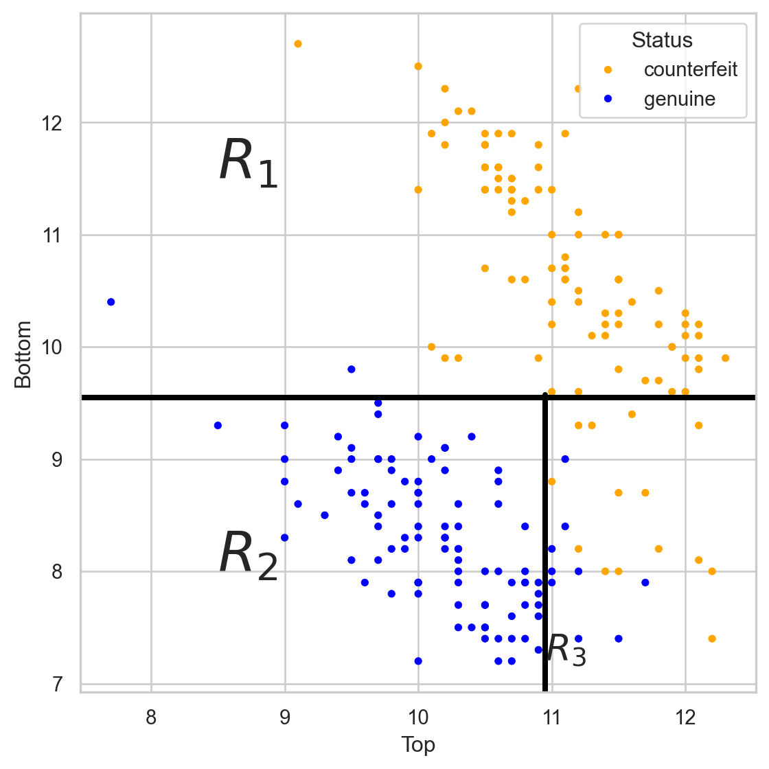
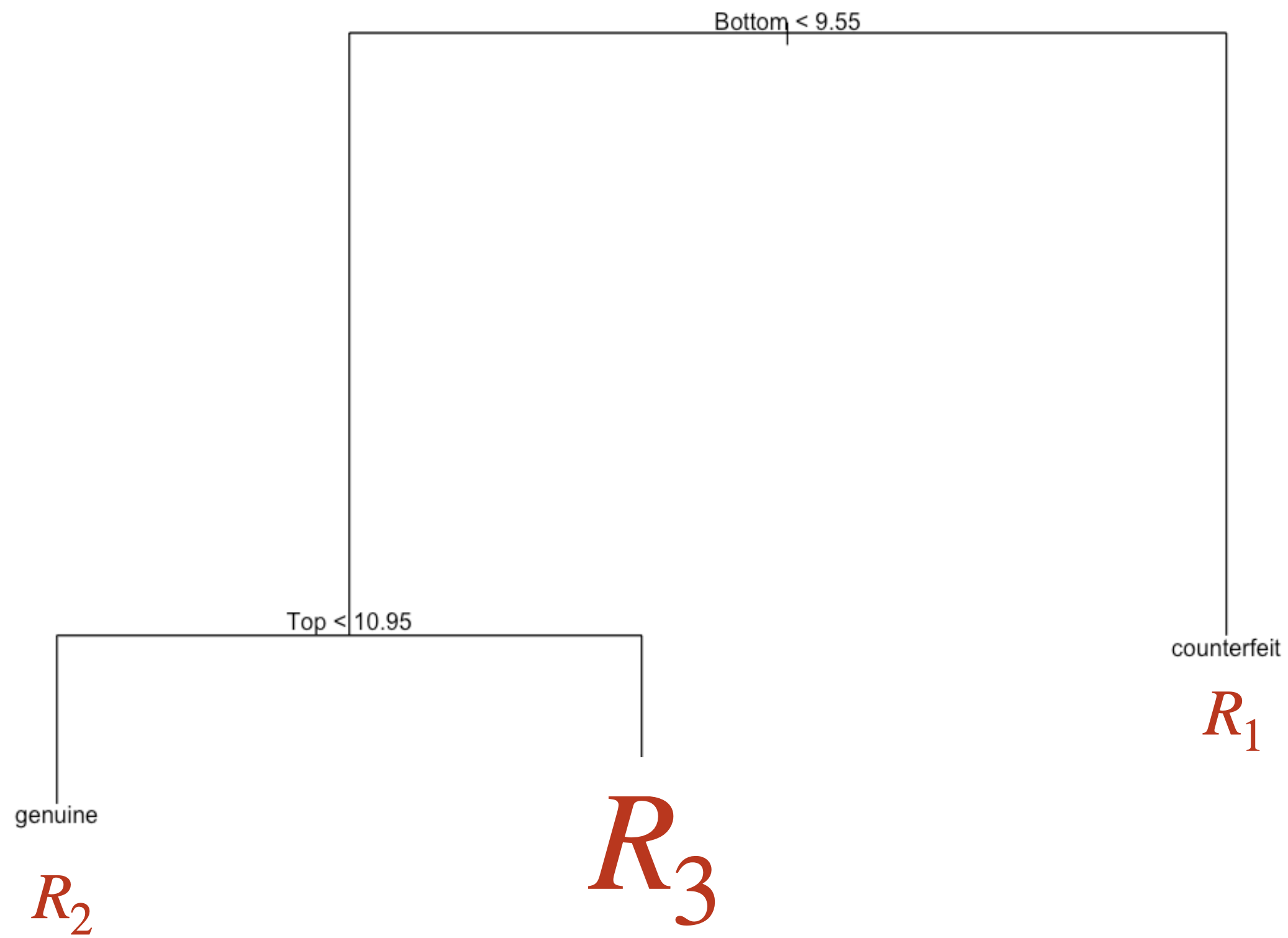
Classification Problems. The response is categorical and involves K different categories. For example, the brand of a product purchased (A, B, C) or whether a person defaults on a debt (yes or no).

The predictors can be numerical or categorical.

Main data science problems

Regression Problems. The response is numerical. For example, a person’s income, the value of a house, or a patient’s blood pressure.

Classification Problems. The response is categorical and involves K different categories. For example, the brand of a product purchased (A, B, C) or whether a person defaults on a debt (yes or no).

The predictors can be numerical or categorical.

Terminology

Recall that

• \(X\) represents a predictor or explanatory variable.
• \(\boldsymbol{X} = (X_1, X_2, \ldots, X_p)\) represents a collection of \(p\) predictors.

Response:

• \(Y\) is a categorical variable that takes 2 categories or classes.

• For example, \(Y\) can take 0 or 1, A or B, no or yes, spam or no spam.

• When classes are strings, they are usually encoded as 0 and 1.

  • The target class is the one for which \(Y = 1\).
  • The reference class is the one for which \(Y = 0\).

Classification algorithms

Classification algorithms use predictor values to predict the class of the response (either target or reference).

That is, for an unseen record, they use predictor values to predict whether the record belongs to the target class or not.

The goal of classification algorithms

Goal: Develop a function \(C(\boldsymbol{X})\) for predicting \(Y = \{0, 1\}\) from \(\boldsymbol{X}\).

To achieve this goal, most algorithms consider functions \(C(\boldsymbol{X})\) that predict the probability that \(Y\) takes the value of 1.

A probability for each class can be very useful for gauging the model’s confidence about the predicted classification.

Example 1

Consider a spam filter where \(Y\) is the email type.

• The target class is spam. In this case, \(Y=1\).
• The reference class is not spam. In this case, \(Y=0\).

Both emails would be classified as spam. However, we would have greater confidence in our classification for the second email.

Technically, \(C(\boldsymbol{X})\) works with the conditional probability:

\[P(Y = 1 | X_1 = x_1, X_2 = x_2, \ldots, X_p = x_p) = P(Y = 1 | \boldsymbol{X} = \boldsymbol{x})\]

In words, this is the probability that \(Y\) takes a value of 1 given that the predictors \(\boldsymbol{X}\) have taken the values \(\boldsymbol{x} = (x_1, x_2, \ldots, x_p)\).

The conditional probability that \(Y\) takes the value of 0 is

\[P(Y = 0 | \boldsymbol{X} = \boldsymbol{x}) = 1 - P(Y = 1 | \boldsymbol{X} = \boldsymbol{x}).\]

Bayes classifier

It turns out that, if we know the true structure of \(P(Y = 1 | \boldsymbol{X} = \boldsymbol{x})\), we can build a good classification function called the Bayes classifier:

\[C(\boldsymbol{X}) = \begin{cases} 1, & \text{if}\ P(Y = 1 | \boldsymbol{X} = \boldsymbol{x}) > 0.5 \\ 0, & \text{if}\ P(Y = 1 | \boldsymbol{X} = \boldsymbol{x}) \leq 0.5 \end{cases}.\]

This function classifies to the most probable class using the conditional distribution \(P(Y | \boldsymbol{X} = \boldsymbol{x})\).

HOWEVER, we don’t (and will never) know the true form of \(P(Y = 1 | \boldsymbol{X} = \boldsymbol{x})\)!

To overcome this issue, we several methods:

• Logistic Regression: Impose an structure on \(P(Y = 1 | \boldsymbol{X} = \boldsymbol{x})\). This was covered in IN1002B.
• Classification Trees: Estimate \(P(Y = 1 | \boldsymbol{X} = \boldsymbol{x})\) directly. What we will cover today.
• Ensemble methods and K-Nearest Neighbours: Estimate \(P(Y = 1 | \boldsymbol{X} = \boldsymbol{x})\) directly. (If time permits).

Once we estimate \(P(Y = 1 | \boldsymbol{X} = \boldsymbol{x})\) using one of these methods, we plug it into the Bayes classifier:

\[\hat{C}(\boldsymbol{X}) = \begin{cases} 1, & \text{if}\ \hat{P}(Y = 1 | \boldsymbol{X} = \boldsymbol{x}) > 0.5 \\ 0, & \text{if}\ \hat{P}(Y = 1 | \boldsymbol{X} = \boldsymbol{x}) \leq 0.5 \end{cases}.\]

where

• \(\hat{P}(Y = 1 | \boldsymbol{X} = \boldsymbol{x})\) is an estimate of \(P(Y = 1 | \boldsymbol{X} = \boldsymbol{x})\).
• \(\hat{C}(\boldsymbol{X})\) is an estimate of the true Bayes Classifier \(C(\boldsymbol{X})\)

Training, Validation, and Test Data

Two datasets

The application of data science algorithms needs two data sets:

• Training data is data that we use to train or construct the approximation \(\hat{C}(\boldsymbol{X})\).

• Test data is data that we use to evaluate the classification performance of \(\hat{C}(\boldsymbol{X})\) only.

A random sample of \(n\) observations.

Use it to construct \(\hat{C}(\boldsymbol{X})\).

Another random sample of \(n_t\) observations, which is independent of the training data.

Use it to evaluate \(\hat{C}(\boldsymbol{X})\).

Validation dataset

In many practical situations, a test dataset is not available. To overcome this issue, we use a validation dataset.

Idea: Apply model to your validation dataset to mimic what will happen when you apply it to test dataset.

Example 2: Identifying Counterfeit Banknotes

Dataset

The data is located in the file “banknotes.xlsx”.

bank_data = pd.read_excel("banknotes.xlsx")
# Set response variable as categorical.
bank_data['Status'] = pd.Categorical(bank_data['Status'])
bank_data.head()

	Status	Left	Right	Bottom	Top
0	genuine	131.0	131.1	9.0	9.7
1	genuine	129.7	129.7	8.1	9.5
2	genuine	129.7	129.7	8.7	9.6
3	genuine	129.7	129.6	7.5	10.4
4	genuine	129.6	129.7	10.4	7.7

How do we generate validation data?

We split the current dataset into a training and a validation dataset. To this end, we use the function train_test_split() from scikit-learn.

The function has three main inputs:

• A pandas dataframe with the predictor columns only.
• A pandas dataframe with the response column only.
• The parameter test_size which sets the portion of the dataset that will go to the validation set.

Create the predictor matrix

We use the function .filter() from pandas to select two predictors: Top and Bottom.

# Set full matrix of predictors.
X_full = bank_data.filter(['Top', 'Bottom'])
X_full.head(4)

	Top	Bottom
0	9.7	9.0
1	9.5	8.1
2	9.6	8.7
3	10.4	7.5

Create the response column

We do the same to extract the column Status from the data frame. We store the result in Y_full.

# Set full matrix of responses.
Y_full = bank_data['Status']
Y_full.head(4)

0    genuine
1    genuine
2    genuine
3    genuine
Name: Status, dtype: category
Categories (2, object): ['counterfeit', 'genuine']

Set the target category

To set the target category in the response we use the get_dummies() function.

# Create dummy variables.
Y_dummies = pd.get_dummies(Y_full, dtype = 'int')

# Select target variable.
Y_target_full = Y_dummies['counterfeit']

# Show target variable.
Y_target_full.head() 

0    0
1    0
2    0
3    0
4    0
Name: counterfeit, dtype: int64

Let’s partition the dataset

# Split the dataset into training and validation.
X_train, X_valid, Y_train, Y_valid = train_test_split(X_full, Y_target_full, 
                                                      test_size = 0.3, 
                                                      stratify = Y_target_full,
                                                      random_state=507134)

• Thanks to the stratify parameter, the function makes a clever partition of the data using the empirical distribution of the response.

• Technically, it splits the data so that the distribution of the response under the training and validation sets is similar.

• Usually, the proportion of the dataset that goes to the validation set is 20% or 30%.

The predictors and response in the training dataset are in the objects X_train and Y_train, respectively. We compile these objects into a single dataset using the function .concat() from pandas. The argument axis = 1 tells .concat() to concatenate the datasets by their rows.

training_dataset = pd.concat([X_train, Y_train], axis = 1)
training_dataset.head(4)

	Top	Bottom	counterfeit
187	10.6	11.4	1
54	10.0	7.9	0
33	10.3	8.4	0
180	10.7	11.4	1

Equivalently, the predictors and response in the validation dataset are in the objects X_valid and Y_valid, respectively.

validation_dataset = pd.concat([X_valid, Y_valid], axis = 1)
validation_dataset.head()

	Top	Bottom	counterfeit
56	10.4	9.2	0
17	9.0	9.0	0
24	10.8	7.4	0
20	10.0	8.4	0
139	10.2	11.8	1

Work on your training dataset

After we have partitioned the data, we work on the training data to develop our predictive pipeline.

The pipeline has two main steps:

1. Data preprocessing.
2. Algorithm development.

Note that all preprocessing techniques will also be applied to the validation and test datasets to prepare it for your algorithm!

Classification Trees

Decision tree

It is a supervised learning algorithm that predicts or classifies observations using a hierarchical tree structure.

Main characteristics:

• Simple and useful for interpretation.

• Can handle numerical and categorical predictors and responses.

• Computationally efficient.

• Nonparametric technique.

Basic idea of a decision tree

Stratify or segment the predictor space into several simpler regions.

How do you build a decision tree?

Building decision trees involves two main procedures:

1. Grow a large tree.

2. Prune the tree to prevent overfitting.

After building a “good” tree, we can predict new observations that are not in the data set we used to build it.

How do we grow a tree?

Using the CART algorithm!

• The algorithm uses a recursive binary splitting strategy that builds the tree using a greedy top-down approach.

• Basically, at a given node, it considers all variables and all possible splits of that variable. Then, for classification, it chooses the best variable and splits it that minimizes the so-called impurity.

We repeat the partitioning process until:

• impurity does not improve in any of the terminal nodes, or
• each terminal node has no less than, say, 5 observations.

What is impurity?

Node impurity refers to the homogeneity of the response classes at that node.

The CART algorithm minimizes impurity between tree nodes.

How do we measure impurity?

There are three different metrics for impurity:

• Misclassification risk.

• Cross entropy.

• Gini impurity index.

p: Proportion of elements in the target class

Mathematically

Let \(p_1\) and \(p_2\) be the proportion of observations in the target and reference class, respectively, in a node.

• Misclassification risk: \(1 - \max\{p_1, p_2\}\)

• Cross entropy: \(- (p_1 \log(p_1) + p_2 \log(p_2))\)

• Gini impurity index: \(p_1(1 - p_1) + p_2(1 - p_2)\)

In Python

In Python, we use the DecisionTreeClassifier() and fit() functions from scikit-learn to train a classification tree.

# We tell Python we want a classification tree
clf = DecisionTreeClassifier(min_samples_leaf= 5, ccp_alpha=0, 
                              random_state=507134)

# We train the classification tree using the training data.
clf.fit(X_train, Y_train)

The parameter min_samples_leaf controls the minimum number of observations in a terminal node, and the cc_alpha controls the tree complexity (to be described later). The parameter random_state allows you to reproduce the same tree in different runs of the Python code.

Plotting the tree

To see the decision tree, we use the plot_tree function from scikit-learn and some commands from matplotlib. Specifically, we use the plt.figure() functions to define the size of the figure and plt.show() to display the figure.

plt.figure(figsize=(6, 6))
plot_tree(clf, feature_names = X_train.columns,
    class_names=["genuine", "counterfeit"], filled=True, rounded=True)
plt.show()

The tree in the predictor space

Estimated conditional probabilities

After training a classification tree, we can calculate the estimated conditional probability \(\hat{P}(Y = 1 | \boldsymbol{X} = \boldsymbol{x})\).

To this end, let

• \(\hat{p}_1(\boldsymbol{x}) = \hat{P}(Y = 1 | \boldsymbol{X} = \boldsymbol{x})\)
• \(\hat{p}_0(\boldsymbol{x}) = 1 - \hat{p}_1(\boldsymbol{x})\)

be the estimated probabilities that \(\boldsymbol{x}\) belongs to class 1 or 0.

Essentially, we calculate \(\hat{p}_1(\boldsymbol{x})\) and \(\hat{p}_0(\boldsymbol{x})\) as follows:

1. Select the region or terminal node where \(\boldsymbol{x}\) belongs.
2. \(\hat{p}_1(\boldsymbol{x})\) is the proportion of observations in that terminal node that belong to class 1. \(\hat{p}_0(\boldsymbol{x})\) is the proportion of observations that belong to class 0.

Visually

Let \((\hat{p}_0(\boldsymbol{x}), \hat{p}_1(\boldsymbol{x}))\) be the estimated probabilities.

Estimated Bayes Classifier

Once we have estimated the conditional probability using the classification tree, we plug it into the Bayes classifier to have our approximated function:

\[\hat{C}(\boldsymbol{x}) = \begin{cases} 1, & \text{if}\ \hat{p}_1(\boldsymbol{x}) > 0.5 \\ 0, & \text{if}\ \hat{p}_1(\boldsymbol{x}) \leq 0.5 \end{cases},\]

where \(\hat{p}_1(\boldsymbol{x})\) depends on the region or terminal node \(\boldsymbol{x}\) falls in.

Simplified decision boundary

Decision boundary logistic regression

Implementation details

• Categorical predictors with unordered levels \(\{A, B, C\}\). We order the levels in a specific way (works for binary and regression problems).

• Predictors with missing values. For quantitative predictors, we use multiple imputation. For categorical predictors, we create a new “NA” level.

• Tertiary or quartary splits. There is not much improvement.

• Diagonal splits (using a linear combination for partitioning). These can lead to improvement, but they impair interpretability.

Classification Metrics

Evaluation

We evaluate a classification tree by classifying observations that were not used for training.

That is, we use the classifier to predict categories in the validation data set using only the predictor values from this set.

In Python, we use the commands:

# Predict classes.
predicted_class = clf.predict(X_valid)

The predict() function generates actual classes to which each observation was assigned.

predicted_class

array([0, 0, 0, 0, 1, 1, 1, 1, 0, 0, 0, 0, 1, 0, 1, 0, 0, 1, 1, 1, 0, 0,
       0, 1, 0, 1, 1, 0, 1, 0, 1, 1, 0, 1, 1, 1, 0, 1, 0, 0, 0, 1, 1, 0,
       0, 0, 1, 0, 1, 0, 0, 0, 1, 1, 1, 1, 0, 1, 1, 1])

The predict_proba() function generates the probabilities used by the algorithm to assign the classes.

# Predict probabilities.
predicted_probability = clf.predict_proba(X_valid)
predicted_probability

array([[1.        , 0.        ],
       [1.        , 0.        ],
       [1.        , 0.        ],
       [1.        , 0.        ],
       [0.        , 1.        ],
       [0.        , 1.        ],
       [0.        , 1.        ],
       [0.        , 1.        ],
       [1.        , 0.        ],
       [1.        , 0.        ],
       [1.        , 0.        ],
       [1.        , 0.        ],
       [0.        , 1.        ],
       [1.        , 0.        ],
       [0.11111111, 0.88888889],
       [0.71428571, 0.28571429],
       [1.        , 0.        ],
       [0.11111111, 0.88888889],
       [0.        , 1.        ],
       [0.        , 1.        ],
       [0.71428571, 0.28571429],
       [1.        , 0.        ],
       [1.        , 0.        ],
       [0.        , 1.        ],
       [1.        , 0.        ],
       [0.        , 1.        ],
       [0.        , 1.        ],
       [1.        , 0.        ],
       [0.        , 1.        ],
       [1.        , 0.        ],
       [0.11111111, 0.88888889],
       [0.        , 1.        ],
       [1.        , 0.        ],
       [0.        , 1.        ],
       [0.        , 1.        ],
       [0.        , 1.        ],
       [1.        , 0.        ],
       [0.        , 1.        ],
       [1.        , 0.        ],
       [1.        , 0.        ],
       [1.        , 0.        ],
       [0.        , 1.        ],
       [0.        , 1.        ],
       [1.        , 0.        ],
       [0.71428571, 0.28571429],
       [1.        , 0.        ],
       [0.11111111, 0.88888889],
       [1.        , 0.        ],
       [0.        , 1.        ],
       [1.        , 0.        ],
       [1.        , 0.        ],
       [1.        , 0.        ],
       [0.        , 1.        ],
       [0.        , 1.        ],
       [0.        , 1.        ],
       [0.        , 1.        ],
       [1.        , 0.        ],
       [0.        , 1.        ],
       [0.        , 1.        ],
       [0.        , 1.        ]])

Confusion matrix

• Table to evaluate the performance of a classifier.

• Compares actual values with the predicted values of a classifier.

• Useful for binary and multiclass classification problems.

In Python

We calculate the confusion matrix using the homonymous function scikit-learn.

# Compute confusion matrix.
cm = confusion_matrix(Y_valid, predicted_class)

# Show confusion matrix.
print(cm)

[[29  1]
 [ 1 29]]

We can display the confusion matrix using the ConfusionMatrixDisplay() function.

CMplot = ConfusionMatrixDisplay(cm, display_labels = ["genuine", "counterfeit"])
CMplot.plot()

Accuracy

It is a simple metric for summarizing the information in the confusion matrix. It is the proportion of correct classifications for both classes, out of the total classifications performed.

In Python, we calculate accuracy using the scikit-learn accuracy_score() function.

accuracy = accuracy_score(Y_valid, predicted_class)
print( round(accuracy, 2) )

0.97

The higher the accuracy, the better the performance of the classification algorithm.

Pruning the tree

In some cases, we can optimize the performance of the tree by pruning it. That is, we collapse two internal (non-terminal) nodes.

To prune a tree, we use an advanced algorithm to measure the contribution of the tree’s branches.

This algorithm minimizes the following function:

\[\text{Missclassification rate of tree} + \alpha (\text{\# terminal nodes}),\]

where \(\alpha\) is a tuning parameter that places greater weight on the number of tree nodes (or size).

• Large values of \(\alpha\) result in small trees with few nodes.

• Small values of \(\alpha\) result in large trees with many nodes.

Apply penalty for large trees

Now, let’s illustrate the pruning technique to find a small decision tree that performs well. To do this, we will train several decision trees using different values of \(\alpha\), which weighs the contribution of the tree branches.

In Python, this is achieved using the cost_complexity_pruning_path() function with the following syntax.

path = clf.cost_complexity_pruning_path(X_train, Y_train)
ccp_alphas = path.ccp_alphas

The ccp_alphas object contains the different values of \(\alpha\) used. To train a decision tree using different \(\alpha\) values, we use the following code that iterates over the values contained in ccp_alphas.

clfs = []
for ccp_alpha in ccp_alphas:
    clf_alpha = DecisionTreeClassifier(min_samples_leaf= 5, 
                                       ccp_alpha=ccp_alpha, random_state=507134)
    clf_alpha.fit(X_train, Y_train)
    clfs.append(clf_alpha)

Now, for each of those trees contained in clfs, we evaluate the performance in terms of accuracy for the training and validation data.

train_scores = [clf.score(X_train, Y_train) for clf in clfs]
validation_scores = [clf.score(X_valid, Y_valid) for clf in clfs]

The .score() function computes the accuracy of a classification tree.

We visualize the results using the following plot.

fig, ax = plt.subplots()
ax.set_xlabel("alpha")
ax.set_ylabel("Accuracy")
ax.set_title("Accuracy vs alpha for training and validation data")
ax.plot(ccp_alphas, train_scores, marker="o", label="train", drawstyle="steps-post")
ax.plot(ccp_alphas, validation_scores, marker="o", label="validation", drawstyle="steps-post")
ax.legend()
plt.show()

Choosing the best tree

We can see that the best \(\alpha\) value for the validation dataset is 0.

To train our new reduced tree, we use the DecisionTreeClassifier() function again with the ccp_alpha parameter set to the best \(\alpha\) value. The object containing this new tree is clf_simple.

# We tell Python that we want a classification tree
clf_simple = DecisionTreeClassifier(ccp_alpha=0, min_samples_leaf= 5)

# We train the classification tree using the training data.
clf_simple.fit(X_train, Y_train)

Once this is done, we can visualize the small tree using the plot_tree() function.

plt.figure(figsize=(6, 6))
plot_tree(clf_simple, feature_names = X_train.columns,
    class_names=["genuine", "counterfeit"], filled=True, rounded=True)
plt.show()

The accuracy of the pruned tree is:

single_tree_Y_pred = clf_simple.predict(X_valid)
accuracy = accuracy_score(Y_valid, single_tree_Y_pred)
print( round(accuracy, 2) )

0.97

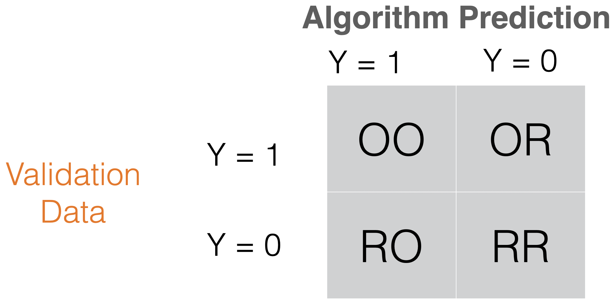
Comments on accuracy

• Accuracy is easy to calculate and interpret.

• It works well when the data set has a balanced class distribution (i.e., cases 1 and 0 are approximately equal).

• However, there are situations in which identifying the target class is more important than the reference class.

• For example, it is not ideal for unbalanced data sets. When one class is much more frequent than the other, accuracy can be misleading.

An example

• Let’s say we want to create a classifier that tells us whether a mobile phone company’s customer will churn next month.

• Customers who churn significantly decrease the company’s revenue. That’s why it’s important to retain these customers.

• To retain that customer, the company will send them a text message with an offer for a low-cost mobile plan.

• Ideally, our classifier correctly identifies customers who will churn, so they get the offer and, hopefully, stay.

• In other words, we want to avoid making wrong decisions about customers who will churn.

• Wrong decisions about loyal customers aren’t as relevant.

• Because if we classify a loyal customer as one who will churn, the customer will get a good deal. They’ll probably pay less but stay anyway.

Another example

• Another example is developing an algorithm (classifier) that can quickly identify patients who may have a rare disease and need a more extensive and expensive medical evaluation.

• The classifier must make correct decisions about patients with the rare disease, so they can be evaluated and eventually treated.

• A healthy patient who is misclassified with the disease will only incur a few extra dollars to pay for the next test, only to discover that the patient does not have the disease.

Classification-specific metrics

To overcome this limitation of accuracy, there are several class-specific metrics. The most popular are:

• Sensitivity or recall

• Precision

• Type I error

These metrics are calculated from the confusion matrix.

Sensitivity or recall = OO/(OO + OR) “How many records of the target class did we predict correctly?”

Precision = OO/(OO + RO) How many of the records we predicted as target class were classified correctly?

In Python, we compute sensitivity and precision using the following commands:

recall = recall_score(Y_valid, predicted_class)
print( round(recall, 2) )

0.97

precision = precision_score(Y_valid, predicted_class)
print( round(precision, 2) )

0.97

Type I error = RO/(RO + RR) “How many of the reference records did we incorrectly predict as targets?”

Unfortunately, there is no simple command to calculate the type-I error in sklearn. To overcome this issue, we must calculate it manually.

# Confusion matrix to compute Type-I error
tn, fp, fn, tp = confusion_matrix(Y_valid, predicted_class).ravel()

# Type-I error rate = False Positive Rate = FP / (FP + TN)
type_I_error = fp / (fp + tn)
print( round(type_I_error, 2) )

0.03

Discussion

• There is generally a trade-off between sensitivity and Type I error.

• Intuitively, increasing the sensitivity of a classifier is likely to increase Type I error, because more observations are predicted as positive.

• Possible trade-offs between sensitivity and Type I error may be appropriate when there are different penalties or costs associated with each type of error.

Disadvantages of decision trees

• Decision trees have high variance. A small change in the training data can result in a very different tree.

• It has trouble identifying simple data structures.

Return to main page