Before we start, let’s import the data science libraries into Python.
import numpy as npimport pandas as pdimport matplotlib.pyplot as pltimport seaborn as snsfrom sklearn.model_selection import train_test_splitfrom sklearn.linear_model import LinearRegressionfrom sklearn.metrics import mean_squared_error, root_mean_squared_error
Here, we use specific functions from the pandas, matplotlib, seaborn and sklearn libraries in Python.
What is a time series?
It is a sequence of observations collected at successive time intervals.
Time series data is commonly used in finance, economics, weather forecasting, signal processing, and many others.
Analyzing time series data helps us understand patterns, trends, and behaviors over time, enabling prediction, anomaly detection, and decision-making.
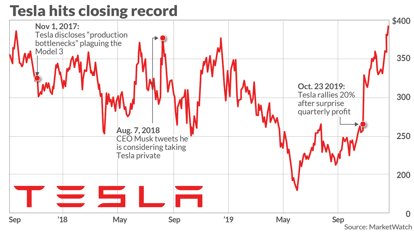
Example 1: Tesla’s stock price
Technically, a time series is a set of observations about a (discrete) predictor \(T\) and a response \(Y\).
Observations of \(Y\) are recorded at the moments or times given by the predictor \(T\).
The special feature of the time series is that the observations of \(Y\) are not independent!
Day
T
Temperature (Y)
Monday
1
10
Tuesday
2
12
Wednesday
3
15
Thursday
4
14
Friday
5
18
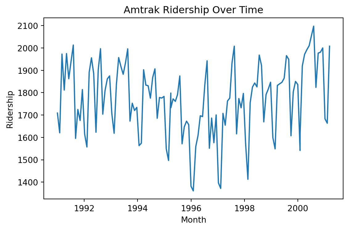
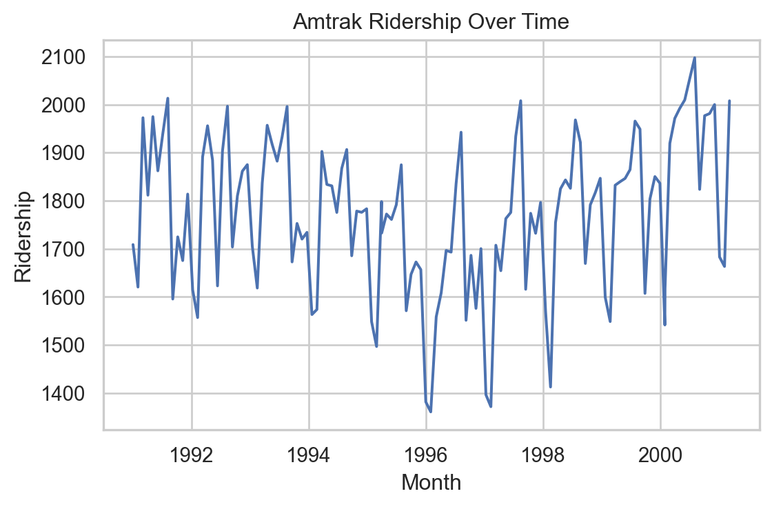
Example 2: Amtrak data
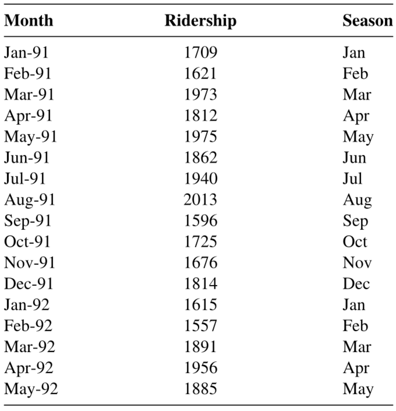
The Amtrak train company in the USA collects data on the number of passengers traveling on its trains.
Records are available from January 1991 to March 2004.
The data is available in “Amtrak.xlsx” on Canvas.
Amtrak_data = pd.read_excel('Amtrak.xlsx')
Amtrak_data.head()
Month
t
Ridership (in 000s)
Season
0
1991-01-01
1
1708.917
Jan
1
1991-02-01
2
1620.586
Feb
2
1991-03-04
3
1972.715
Mar
3
1991-04-04
4
1811.665
Apr
4
1991-05-05
5
1974.964
May
Time series plot in Python
We can create a line graph to visualize the evolution of Amtrak train ridership over time using lineplot from seaborn.
Code
plt.figure(figsize=(6, 4))sns.lineplot(x='Month', y='Ridership (in 000s)', data = Amtrak_data)plt.xlabel('Month')plt.ylabel('Ridership')plt.title('Amtrak Ridership Over Time')plt.tight_layout()plt.show()
Informative Series
An informative time series is a series that contains patterns that we can use to predict future values of the series.
The three possible patterns are:
Trend: the series has an increasing/decreasing behavior.
Seasonality: the series has a repeating cyclical pattern in its values.
Autocorrelation: the series follows a pattern that can be described by previous values of the series.
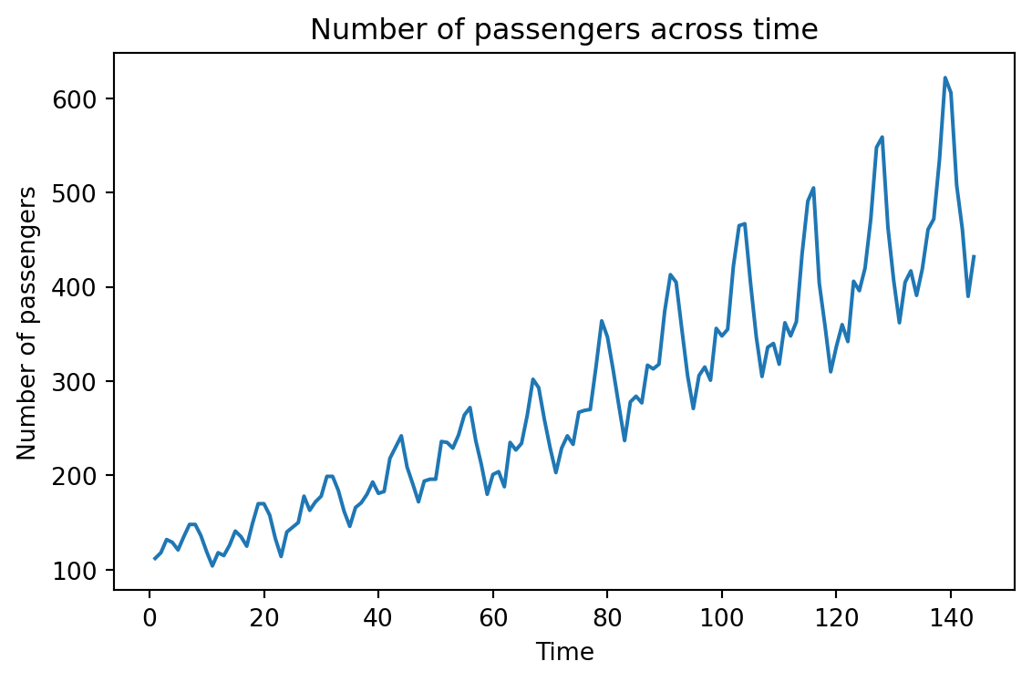
Example 3: Airline data
This series has an upper trend.
This series has cyclical patterns in its values.
Although not immediately visible, we can use the previous values of the series to describe the future ones.
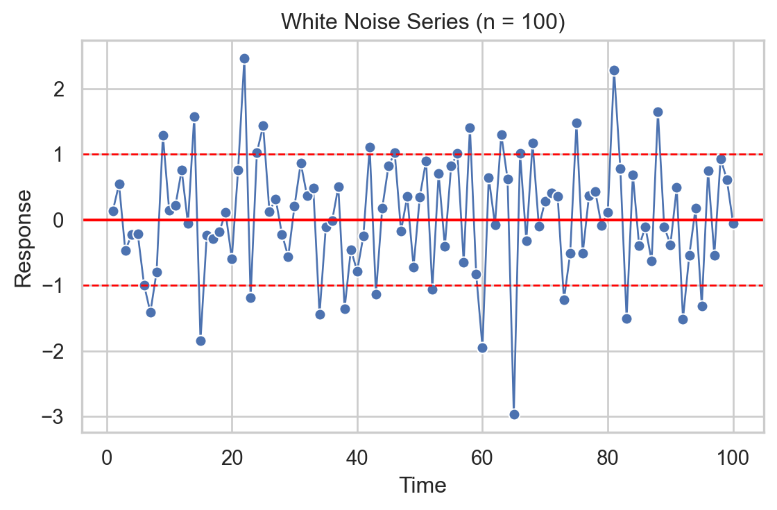
Non-informative series: White noise
White noise is a series whose values, on average, are 0 and have a constant variation.
Its values are also independent of each other.
It is used to describe random or natural error.
Linear Regression Model for Time Series
Linear regression model
The linear regression model is useful for capturing patterns in a time series. In this context, the model takes the form:
\[\hat{Y}_i = \hat{\beta}_0 + \hat{\beta}_1 T_i\]
Where \(i = 1, \ldots, n_t\) is the index of the \(n_t\) training data.
\(\hat{Y}_i\) is the prediction of the actual value of the response \(Y_i\)at time\(T_i\).
Trend
The trend of the time series is captured by the value of \(\hat{\beta}_1\) at
\[\hat{Y}_i = \hat{\beta}_0 + \hat{\beta}_1 T_i\]
If \(\hat{\beta}_1\) is positive, the series has an upward trend.
If \(\hat{\beta}_1\) is negative, the series has a downward trend.
The values of \(\hat{\beta}_0\) and \(\hat{\beta}_1\) are obtained using the least squares method.
Model evaluation
Remember that the errors of the linear regression model (\(e_i = Y_i - \hat{Y}_i\)) must meet three conditions:
On average, they must be equal to 0.
They must have the same dispersion or variability.
They must be independent of each other.
In the context of time series, this means that the model errors\(e_i\) must behave like white noise that contains no patterns.
Example 2: Amtrak data (cont.)
Let’s fit a linear regression model to the ridership data from Amtrak.
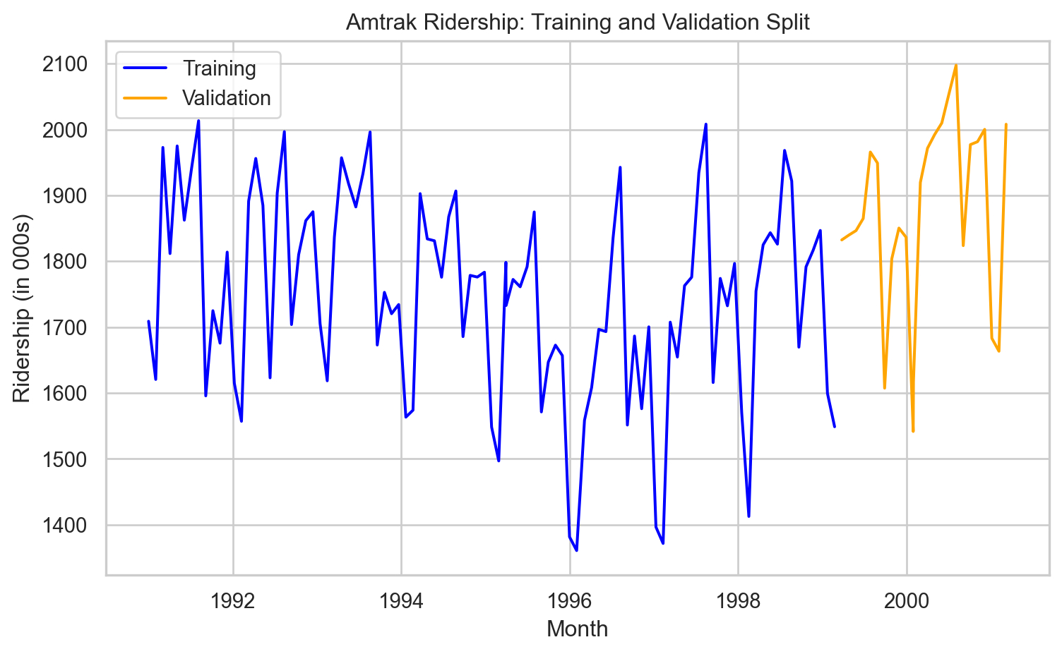
Creating a train and a validation data
In time series, the order of the data matters because each observation is tied to a specific point in time.
Because of this, we cannot randomly split the data using a function like train_test_split().
Doing so might result in a situation where the model learns from future values to predict past ones—which doesn’t make sense and would lead to overly optimistic performance.
Instead, we want to train the model on earlier time periods and test it on later ones.
To this end, we use the code below.
# Define the split pointsplit_ratio =0.8# 80% train, 20% validationsplit_point =int(len(Amtrak_data) * split_ratio)# Split the dataAmtrak_train = Amtrak_data[:split_point]Amtrak_validation = Amtrak_data[split_point:]
This code ensures that the training data always comes before the validation data in time, preserving the temporal order. The proportion of data that goes to training is set using split_ratio.
Fit linear regression model
We first set the predictor and response.
# Set predictor.X_train = Amtrak_train.filter(['t'])# Set response.Y_train = Amtrak_train.filter(['Ridership (in 000s)'])
Next, we fit the model using LinearRegression() and fit() from scikit-learn.
# 1. Create linear regression model.LRmodelAmtrak = LinearRegression()# 2. Fit the model to the training data.LRmodelAmtrak.fit(X_train, Y_train)
Let’s inspect the estimated coefficient for the predictor (time).
print(LRmodelAmtrak.coef_)
[[-1.2818326]]
And the intercept.
print(LRmodelAmtrak.intercept_)
[1810.77686661]
The estimated model then is:
\[\hat{Y}_i = 1810.777 - 1.281 T_i.\]
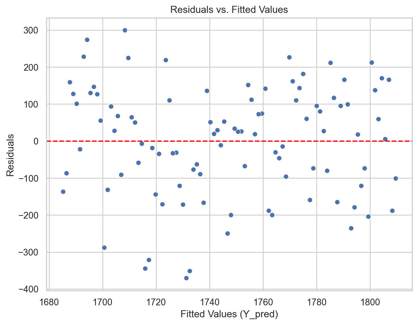
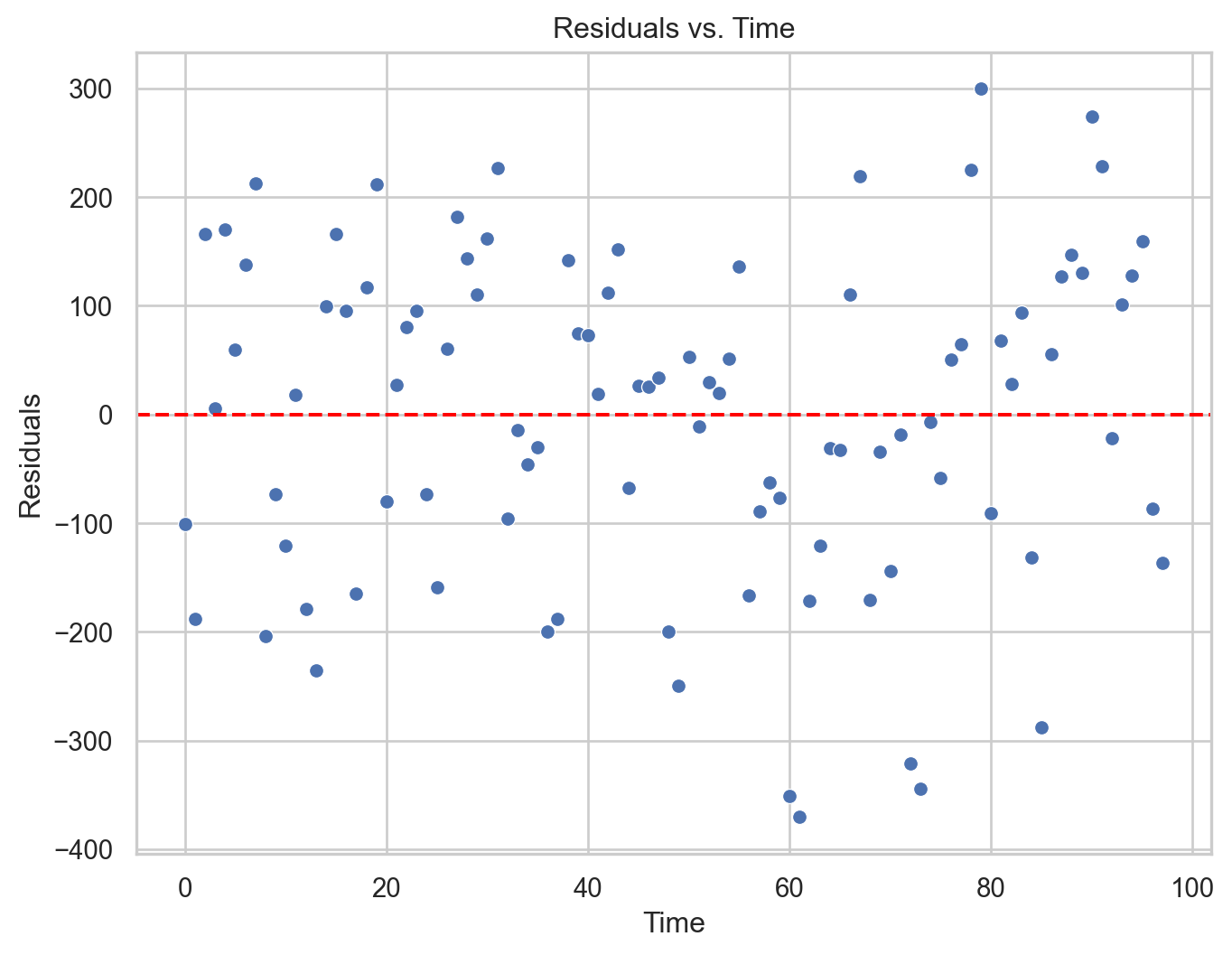
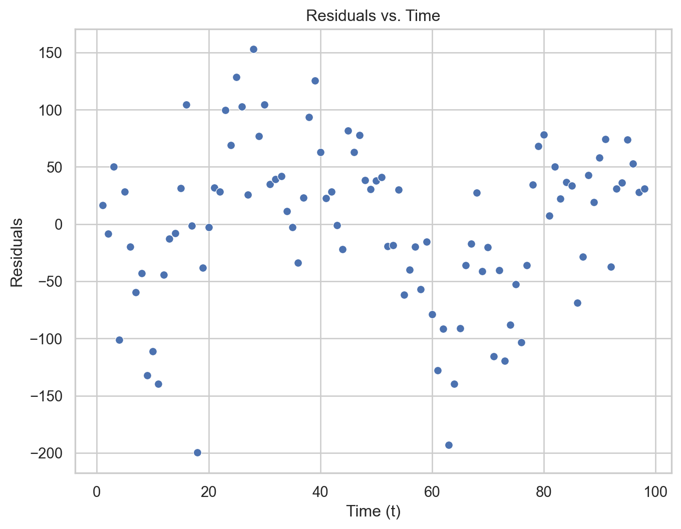
Residual analysis
We can validate the model using a residual analysis on the training data. To this end, we first compute the predicted values and residuals of the model.
Remember that we are using + Y_train*0 to visualize the objects fitted and residuals effectively.
Code
# Residual vs Fitted Values Plotplt.figure(figsize=(8, 6))sns.scatterplot(data = residual_data, x ="Fitted", y ="Residuals")plt.axhline(y=0, color='red', linestyle='--')plt.xlabel("Fitted Values (Y_pred)")plt.ylabel("Residuals")plt.title("Residuals vs. Fitted Values")plt.show()
Code
plt.figure(figsize=(8, 6))sns.scatterplot(data = residual_data, x ="Time", y ="Residuals")plt.axhline(y=0, color='red', linestyle='--')plt.xlabel("Time")plt.ylabel("Residuals")plt.title("Residuals vs. Time")plt.show()
The model is more flexible than that
If necessary, the linear regression model can be extended to capture quadratic relationships. For this, the model takes the following form:
Where \(T^{2}_i\) is the squared value of the time index.
\(\hat{\beta}_2\) is a term that captures possible curvature in the time series.
In Python
To include a quadratic term, we must augment our predictor matrix with an additional column. The following code shows how to augment X_full by the square of the Amtrak_data['t'] column. This is done using the pandas.concat() function. The resulting matrix is stored in X_quad.
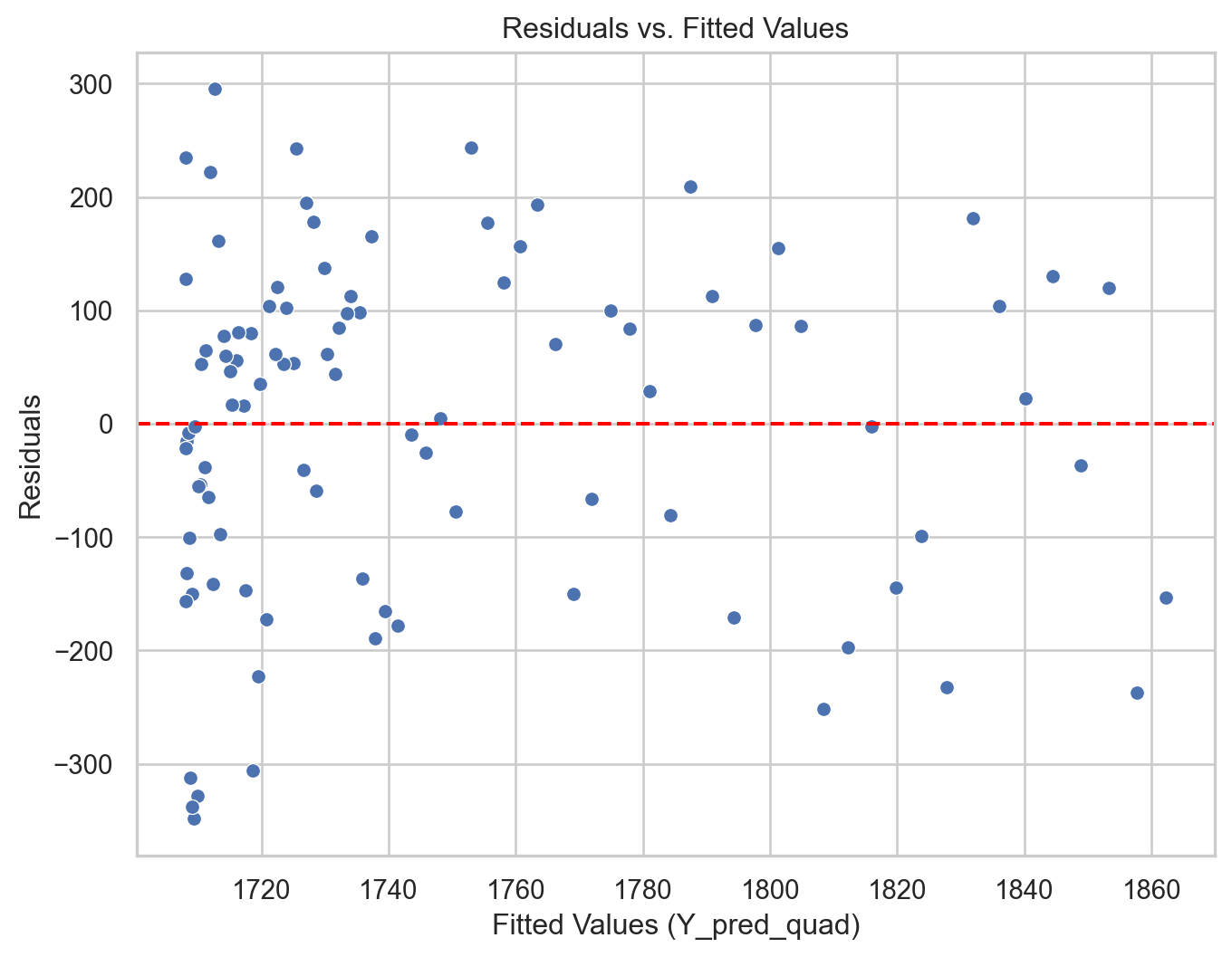
# Remember to use the same `X_quad`Y_pred_quad = QuadmodelAmtrak.predict(X_quad) + Y_train*0residuals_quad = Y_train - Y_pred_quad# Construct a pandas data.frameresidual_data_quad = pd.DataFrame()residual_data_quad["Fitted"] = Y_pred_quadresidual_data_quad["Residuals"] = residuals_quadresidual_data_quad["Time"] = residuals_quad.indexplt.figure(figsize=(8, 6))sns.scatterplot(data = residual_data_quad, x ="Fitted", y ="Residuals")plt.axhline(y=0, color='red', linestyle='--')plt.xlabel("Fitted Values (Y_pred_quad)")plt.ylabel("Residuals")plt.title("Residuals vs. Fitted Values")plt.show()
Code
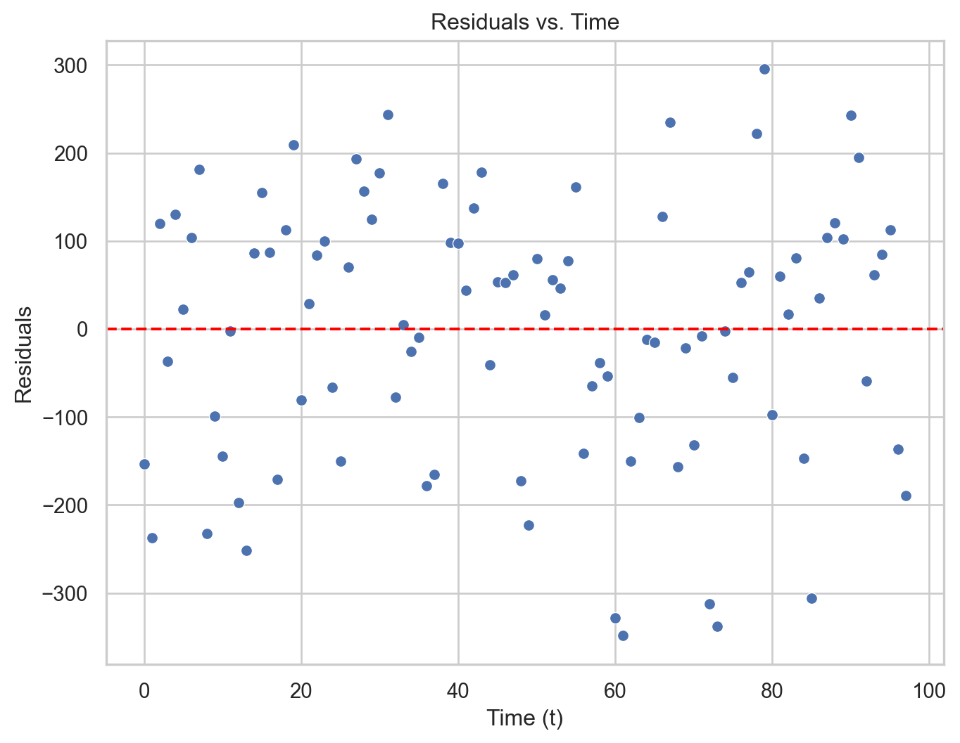
plt.figure(figsize=(8, 6))sns.scatterplot(data = residual_data_quad, x ="Time", y ="Residuals")plt.axhline(y=0, color='red', linestyle='--')plt.xlabel("Time (t)")plt.ylabel("Residuals")plt.title("Residuals vs. Time")plt.show()
Model evaluation using validation data
Remember that another way to evaluate the performance of a model is using the \(\text{MSE}_v\) or \(\text{RMSE}_v\) on the validation data.
To this end, we need some Python objects.
# Set predictor.X_valid = Amtrak_validation.filter(['t'])# Set response.Y_valid = Amtrak_validation.filter(['Ridership (in 000s)'])
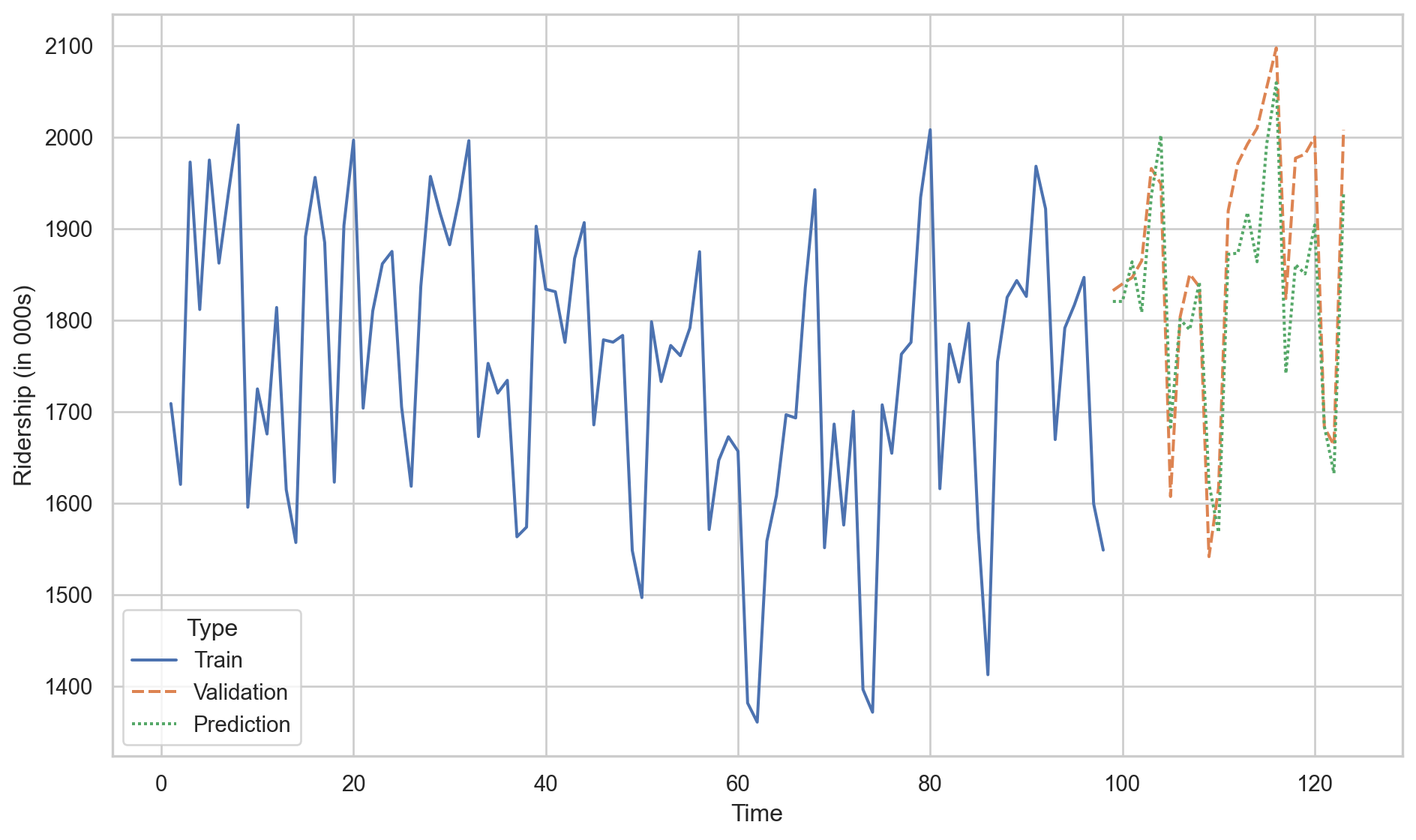
Let’s compute the \(\text{RMSE}_v\) for the linear regression model.
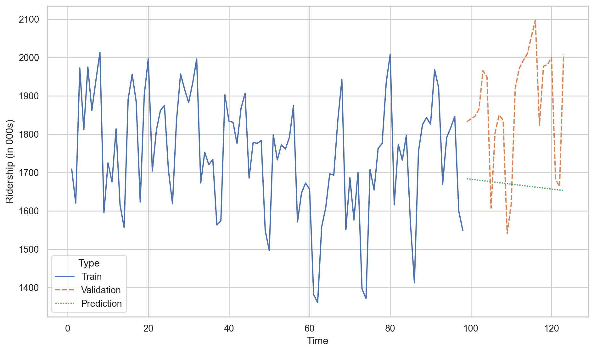
We conclude that the linear model with a quadratic term is better than the linear regression model because the \(\text{RMSE}_v\) of the former is smaller than for the latter.
Predictions of linear model.
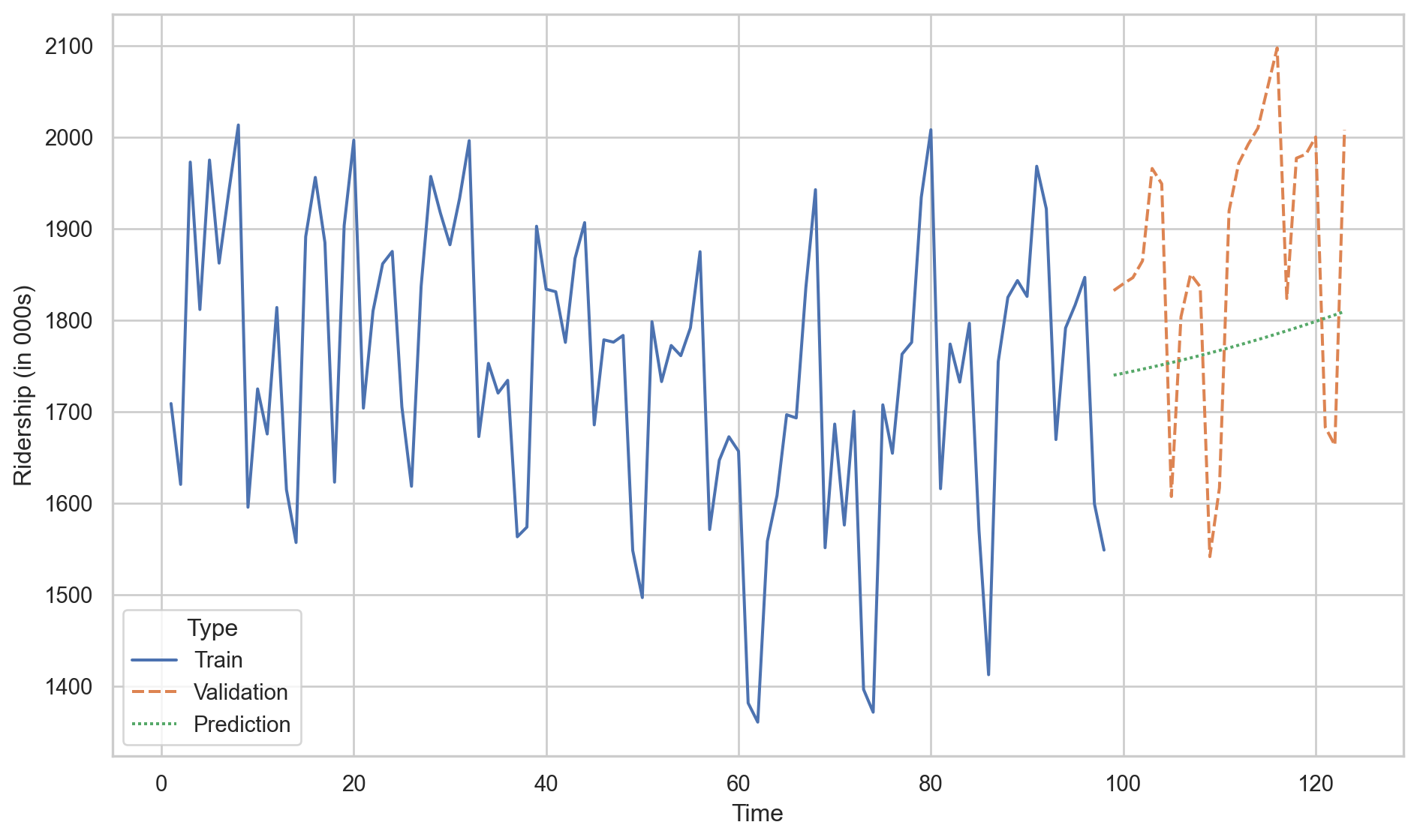
Predictions of linear model with quadratic trend.
Activity (solo mode)
The Office of Transportation Statistics of the Innovative Research and Technology Administration conducted a study to assess the impact of the September 11, 2001, terrorist attack on U.S. transportation. The report analyzes monthly passenger movement data from January 1990 to May 2004. Time series data are provided for (1) Real Revenue Passenger Miles Traveled (Air RPM), (2) Rail Passenger Miles Traveled (Rail PM), and (3) Car Miles Traveled (VMT).
In this activity, you will fit different linear regression models to data in the file “Sept11Travel.xlsx” in CANVAS.
Identifying Heteroskedasticity
Heteroskedasticity arises when the dispersion of model errors is not constant over time.
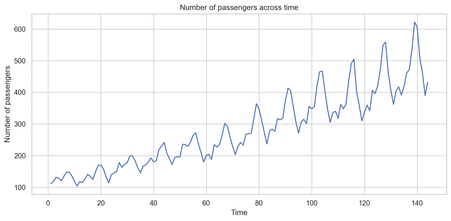
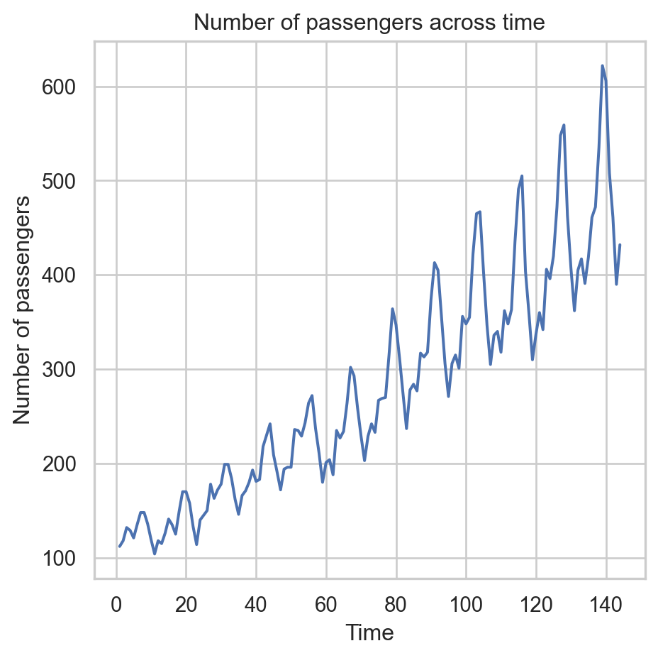
To see it, let’s go back to the Airline data, which contains the number of passengers of an international airline per month between 1949 and 1960.
Airline_data = pd.read_excel("Airline.xlsx")
Airline_data.head()
T
Number of passengers
0
1
112
1
2
118
2
3
132
3
4
129
4
5
121
For illustrative purposes, we will not split the time series into training and validation datasets.
Code
plt.figure(figsize=(10, 5))sns.lineplot(x='T', y='Number of passengers', data = Airline_data)plt.xlabel('Time')plt.ylabel('Number of passengers')plt.title('Number of passengers across time')plt.tight_layout()plt.show()
Let’s fit a linear regression model.
# Set predictor.X_full = Airline_data.filter(['T'])# Set response.Y_full = Airline_data.filter(['Number of passengers'])# 1. Create linear regressionLRmodelAirline = LinearRegression()# 2. Fit the modelLRmodelAirline.fit(X_full, Y_full)
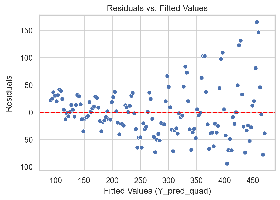
Residual analysis
Heteroskedasticity: Dispersion of the residuals increases with the predicted value.
Code
# Remember to use the same `X_quad`Y_pred = LRmodelAirline.predict(X_full) + Y_full*0residuals = Y_full - Y_pred# Construct a pandas data.frameresidual_data = pd.DataFrame()residual_data["Fitted"] = Y_predresidual_data["Residuals"] = residualsresidual_data["Time"] = residuals.indexplt.figure(figsize=(6, 4))sns.scatterplot(data = residual_data, x ="Fitted", y ="Residuals")plt.axhline(y=0, color='red', linestyle='--')plt.xlabel("Fitted Values (Y_pred_quad)")plt.ylabel("Residuals")plt.title("Residuals vs. Fitted Values")plt.show()
Solution
If we identify heteroskedasticity in the regression model errors, we have several transformation options for our original series.
A common transformations to the time series \(Y_i\) is the Natural Logarithm
If the original time series contains negative values, it can be lagged by adding the negative of its minimum value.
In Python
The easiest way to apply the logarithm in Python is to use the log() function from the numpy library
log_Y_full = np.log( Y_full )
Now, the response to use is in log_Y_full.
The steps to fit a linear regression model are similar.
# 1. Create linear regressionLRmodelAirlineTransformed = LinearRegression()# 2. Fit the modelLRmodelAirlineTransformed.fit(X_full, log_Y_full)
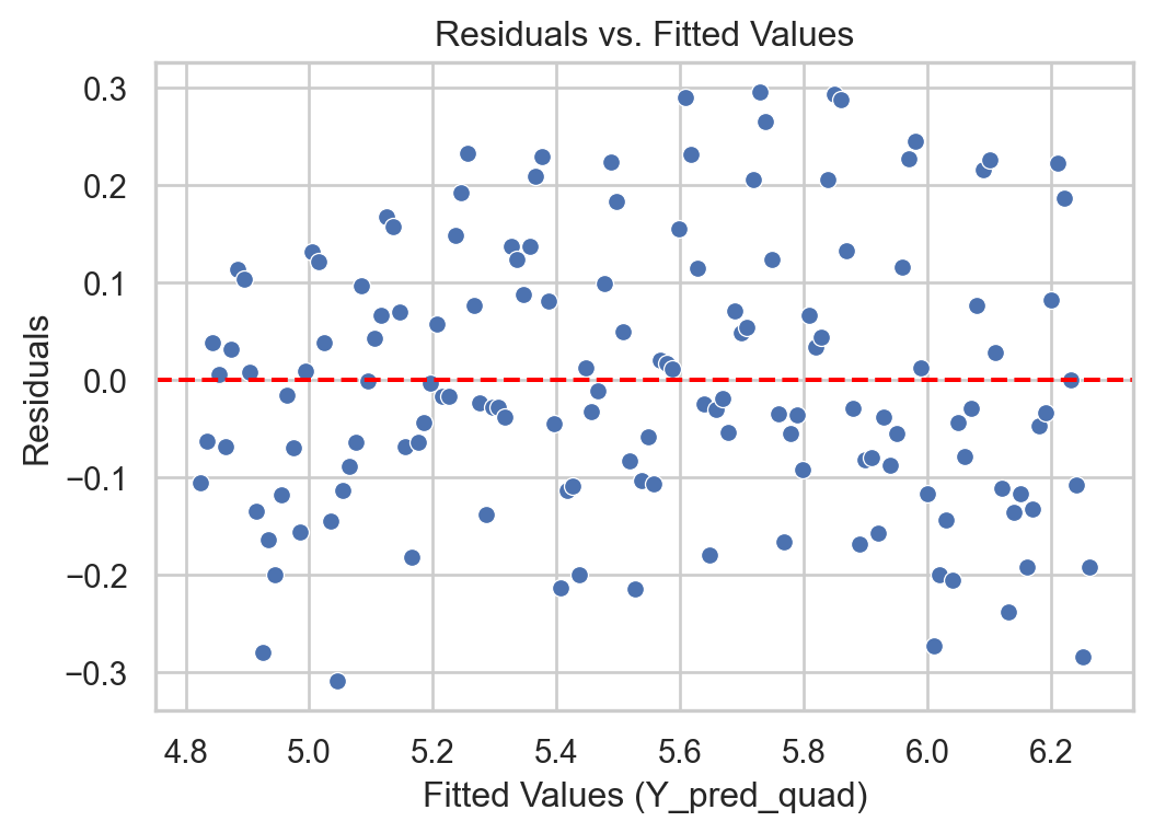
Residual analysis
With transformation
Code
# Remember to use the same `X_quad`Y_pred_log = LRmodelAirlineTransformed.predict(X_full) + log_Y_full*0residuals_log = log_Y_full - Y_pred_log# Construct a pandas data.frameresidual_data_log = pd.DataFrame()residual_data_log["Fitted"] = Y_pred_logresidual_data_log["Residuals"] = residuals_logresidual_data_log["Time"] = residuals_log.indexplt.figure(figsize=(6, 4))sns.scatterplot(data = residual_data_log, x ="Fitted", y ="Residuals")plt.axhline(y=0, color='red', linestyle='--')plt.xlabel("Fitted Values (Y_pred_quad)")plt.ylabel("Residuals")plt.title("Residuals vs. Fitted Values")plt.show()
Without transformation
Code
# Remember to use the same `X_quad`Y_pred = LRmodelAirline.predict(X_full) + Y_full*0residuals = Y_full - Y_pred# Construct a pandas data.frameresidual_data = pd.DataFrame()residual_data["Fitted"] = Y_predresidual_data["Residuals"] = residualsresidual_data["Time"] = residuals.indexplt.figure(figsize=(6, 4))sns.scatterplot(data = residual_data, x ="Fitted", y ="Residuals")plt.axhline(y=0, color='red', linestyle='--')plt.xlabel("Fitted Values (Y_pred_quad)")plt.ylabel("Residuals")plt.title("Residuals vs. Fitted Values")plt.show()
What do I do if the transformation doesn’t work?
If the log transformation doesn’t significantly reduce heteroskedasticity, there are models for modeling variance called GARCH.
You can find literature on these models and their software implementations in a time series textbook such as Time Series Analysis with Applications in R by Cryer and Chan.
Models with Seasonality
Seasonality
Seasonality refers to repetitive or cyclical behavior that occurs with a constant frequency.
Examples:
Demand for winter clothing
Demand for tourist travel
Amount of rainfall throughout the year.
Capturing seasonality
The linear regression model can be extended to capture seasonal patterns in the time series.
To do this, an additional categorical predictor is created that indicates the season to which each data item belongs.
The additional categorical predictor is transformed into several auxiliary numerical predictors.
Analyzing seasonal series in Python
Consider the data in Amtrak_train with the additional predictor of Season to model seasonality.
Month
t
Ridership (in 000s)
Season
0
1991-01-01
1
1708.917
Jan
1
1991-02-01
2
1620.586
Feb
2
1991-03-04
3
1972.715
Mar
3
1991-04-04
4
1811.665
Apr
4
1991-05-05
5
1974.964
May
To fit a linear regression model with a categorical variable like Season, we must transform the text categories into numbers. To do this, we use dummy variables constructed using the following commands.
The matrix above contains one column for each month. Each column indicates the observations that belong to the month of the column. For example, the column Apr has the values 0 and 1. The value 1 indicates that the corresponding observation belongs to the month of April. A 0 indicates otherwise.
Apr
Aug
Dec
Feb
Jan
Jul
Jun
Mar
May
Nov
Oct
Sep
0
0
0
0
0
1
0
0
0
0
0
0
0
1
0
0
0
1
0
0
0
0
0
0
0
0
2
0
0
0
0
0
0
0
1
0
0
0
0
3
1
0
0
0
0
0
0
0
0
0
0
0
Unfortunately, we cannot use the matrix as is in the linear regression model due to multicollinearity issues. Technically, this happens because if you add all the columns, the resulting column is a column of 1s, which is already used by the intercept. Therefore, you cannot fit a model with the intercept and all the columns of the dummy variables.
To solve this problem, we arbitrarily remove a column from the matrix above. For example, let’s remove Dec.
dummy_data = dummy_data.drop(["Dec"], axis =1)
Now, let’s build the complete matrix of predictors, including the column for time, time squared, and the dummy variables.
Next, we fit the model with all the terms in the matrix above.
# 0. Ensure that we have the response in `Y_full`.Y_train = Amtrak_train['Ridership (in 000s)']# 1. Create linear regression model.SeasonmodelAmtrak = LinearRegression()# 2. Fit the linear regression model.SeasonmodelAmtrak.fit(X_quad_season, Y_train)
Despite their simplicity and versatility, linear regression models are not the best for describing a time series.
This is because they do not assume a dependency between consecutive values in the time series. That is, they do not use the fact that, for example, \(Y_1\) can help us predict \(Y_2\), and \(Y_2\) can help us predict \(Y_3\), etc.
Models that help us use past observations to predict future values of the response variable \(Y\) are autoregressive models.
Yogi Berra
It’s though to make predictions, especially about the future.