Tools for Data Manipulation

IN2039: Data Visualization for Decision Making

Alan R. Vazquez

Department of Industrial Engineering

Agenda

Introduction to R
Reading data with readxl
Data manipulation with dplyr

Introduction to R

R

A versatile programming language.
It is free!
It is widely used for data cleaning, data visualization, and data modelling.
It can be extended with packages (libraries) developed by other users.

Google Colab

Google’s free cloud collaboration platform for creating R documents.

Run R and collaborate on Jupyter notebooks for free.
Harness the power of GPUs for free to accelerate your data science projects.
Easily save and upload your notebooks to Google Drive.

Let’s try a command in R

What do you think will happen if we run this command?

print("Hello world!")

[1] "Hello world!"

Let’s try another command

What do you think will happen if we run this command?

sum(1, 5, 10)

[1] 16

Use R as a basic calculator

5 + 1

[1] 6

10 - 3

[1] 7

2 * 4

[1] 8

9 / 3

[1] 3

Comments

Sometimes we write things in the coding window that we want R to ignore. These are called comments and start with #.

R will ignore the comments and just execute the code.

# you can put whatever after #
# for example... blah blah blah

Introduction to functions in R

One of the cool things about R is that there are many built-in commands you can use. These are called functions.

Functions have two basic parts:

The first part is the name of the function (for example, sum).
The second part is the input to the function, which goes inside the parentheses (sum(1, 5, 15)).

R is strict

R, like all programming languages, is very strict. For example, if you write

sum(1, 100)

[1] 101

it will tell you the answer, 101.

But if you write

Sum(1, 100)

Error in Sum(1, 100): could not find function "Sum"

with the “s” capitalized, R will act like it has no idea what we are talking about!

Save your work in R objects

Virtually anything, including the results of any R function, can be saved in an object.

This is accomplished by using an assignment operator, which can be an equal symbol (=) or a leftward symbol (<-).

You can make up any name you want for a R object. However, there are two basic rules for this:

It has to be different from a function name in R.
It has to be specific possible yet succinct.

For example

# This code will assign the number 18
# to the object called my_favorite_number

my_favorite_number = 18

After running this code, nothing happens. But if we run the object on its own, we can see what’s inside it.

my_favorite_number

[1] 18

You can also use print(my_favorite_number).

Vectors

So far we have used R objects to store a single number. But in data visualization we are dealing with multiple numbers or observations.

A R object can also store a complete set of numbers, called a vector.

You can think of a list as a vector of numbers (or values).

The c() command can be used to combine several individual values into a list.

For example

This code creates two vectors:

my_vector = c(1, 2, 3, 4, 5)
my_vector_2 = c(10, 10, 10, 10, 10)

Let’s see their content:

my_vector

[1] 1 2 3 4 5

my_vector_2

[1] 10 10 10 10 10

Operations

We can do simple operations with vectors. For example, we can sum all the elements of a list.

my_vector = c(1, 2, 3, 4, 5)
sum(my_vector)

[1] 15

Indexing

We can index a position in the vector using square brackets with a number like this: [1].

So, if we wanted to print the contents of the first position in my_vector, we could write

my_vector[1]

[1] 1

In contrast with Python, the first element of an R vector is indexed using 1.

A little more about R objects

You can think of R objects as containers that hold values.

A R object can hold a single value, or it can hold a group of values (as in a vector).

So far, we’ve only put numbers into R objects.

R objects can actually contain three types of values: numbers, characters, and booleans.

Character values

Characters are made up of text, such as words or sentences. An example of a list with characters as elements is:

many_greetings = c("hi", "hello", "hola", "bonjour", "ni hao", "merhaba")
many_greetings

[1] "hi"      "hello"   "hola"    "bonjour" "ni hao"  "merhaba"

It is important to know that numbers can also be treated as characters, depending on the context.

For example, when 20 is enclosed in quotes ("20") it will be treated as a character value, even though it encloses a number in quotes.

Boolean values

Boolean values are True or False.

We may have a question like:

Is the first element of the vector many_greetings "hola"?

We can ask R to find out and return the answer True or False.

many_greetings[1] == "hola"

[1] FALSE

Logical operators

Most of the questions we ask R to answer with True or False involve comparison operators like >, <, >=, <=, and ==.

The double == sign checks whether two values are equal. There is even a comparison operator to check whether values are not equal: !=.

For example, 5 != 3 is a True statement.

Common logical operators

> (larger than)
>= (larger than or equal to)
< (smaller than)
<= (smaller than or equal to)
== (equal to)
!= (not equal to)

Programming culture: Trial and error

The best way to learn programming is to try things out and see what happens. Write some code, run it, and think about why it didn’t work.

There are many ways to make small mistakes in programming (for example, typing a capital letter when a lowercase letter is needed).

We often have to find these mistakes through trial and error.

R libraries

Libraries are the fundamental units of reproducible R code. They include reusable R functions, documentation describing how to use them, and sample data.

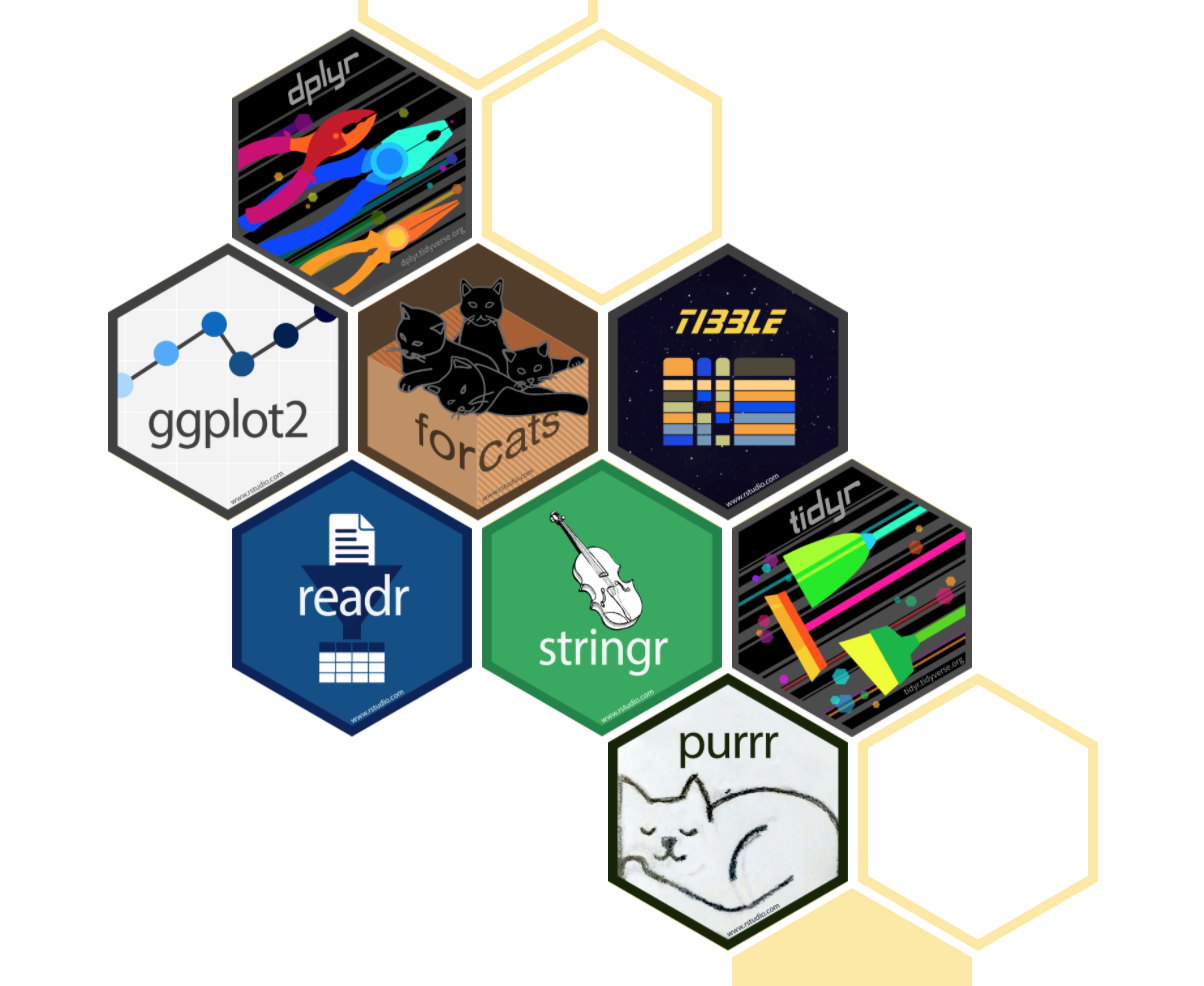
In this course, we will be working mostly with the following libraries for data manipulation:

readxl for reading data.
dplyr for data manipulation and wrangling
tidyr for structuring data.

Reading data with readxl

Loading data in R

In this course, we will assume that data is stored in an Excel file. As an example, let’s use the file penguins.xlsx.

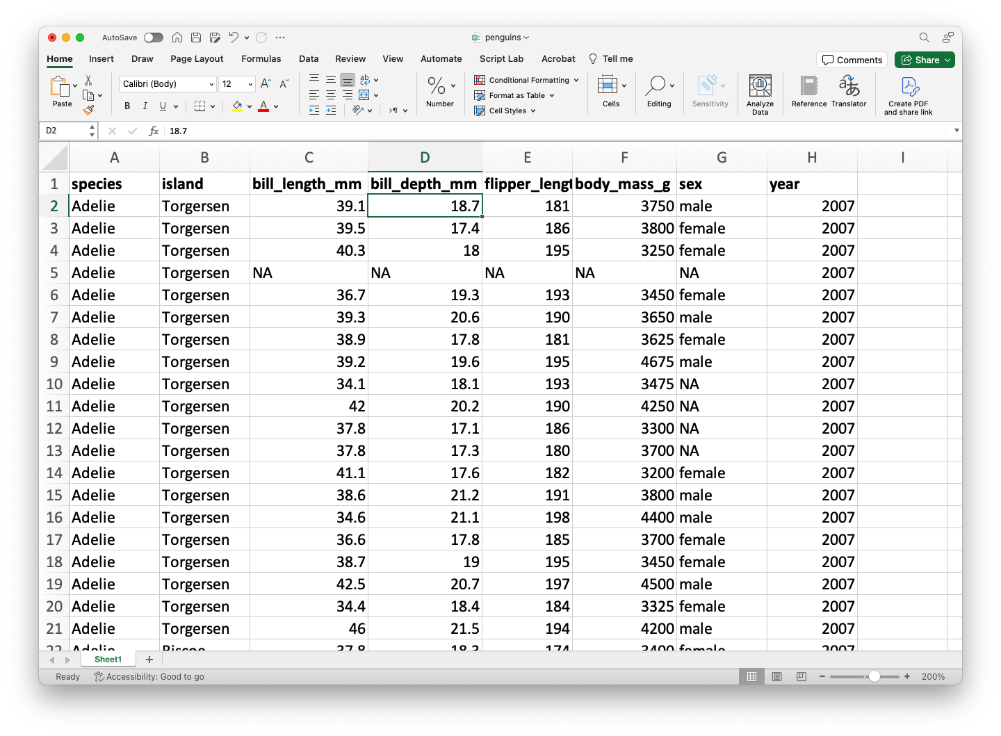
The file must be previously uploaded to Google Colab.

The dataset penguins.xlsx contains data from penguins living in three islands.

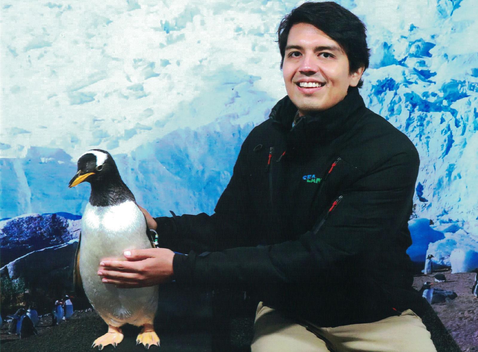
Alan Vazquez with a gentoo penguin

readxl library

To load data into R, we’ll use the library called readxl. Fortunately, this library comes pre-installed in Google Colab.

However, we need to inform Google Colab that we want to use readxl and its functions. We load the library into R using the following command.

library(readxl)

Loading data using readxl

The following code shows how to read the data in the file “penguins.xlsx” into R.

# Load the Excel file into R.
penguins_data = read_excel("penguins.xlsx")

The function `head()`

The function head() allows you to print the first 6 rows of a data frame.

# Print the first 4 rows of the dataset.
head(penguins_data)

# A tibble: 6 × 8
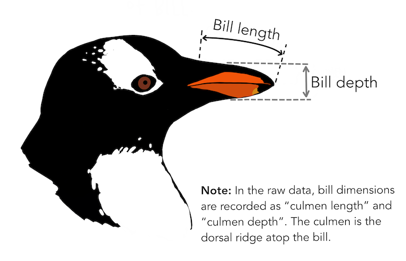
  species island    bill_length_mm bill_depth_mm flipper_length_mm body_mass_g
  <chr>   <chr>              <dbl>         <dbl>             <dbl>       <dbl>
1 Adelie  Torgersen           39.1          18.7               181        3750
2 Adelie  Torgersen           39.5          17.4               186        3800
3 Adelie  Torgersen           40.3          18                 195        3250
4 Adelie  Torgersen           NA            NA                  NA          NA
5 Adelie  Torgersen           36.7          19.3               193        3450
6 Adelie  Torgersen           39.3          20.6               190        3650
# ℹ 2 more variables: sex <chr>, year <dbl>

Mini-activity (solo mode)

Open the following Google Colab link: https://drive.google.com/file/d/1kS1_M-wLRc9BDRAadV_K6yosNK0XF9qi/view?usp=sharing
Copy the notebook to your drive.
Answer the questions.

Data manipulation with dplyr

A New Library: dplyr

dplyr allows you to manipulate data and generate statistical summaries.
It is part of a collection of data science packages called tidyverse.
https://dplyr.tidyverse.org/

Load it to Google Colab with the following code.

library(dplyr)

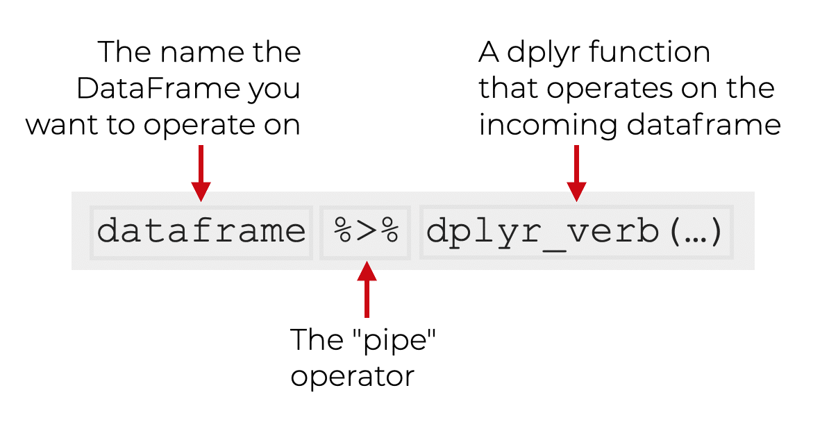
pipe

One of the most important commands of dplyr is pipe, which is executed using the operator %>%. This operator sends an object to a calling function or expression.

The grammar for using pipe is as follows:

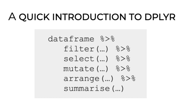
dplyr’s verbs

dplyr is a data manipulation grammar that provides a set of verbs (functions) to solve the most common data manipulation challenges:

filter() selects observations based on their values.
select() selects variables based on their names.
mutate() adds new variables that are functions of existing variables.
arrange() changes the order of rows.
summarise() reduces multiple values to a single numerical summary.

To practice, we will use the dataset penguins_data.

Filter observations with `filter()`

We can filter the data to obtain penguins with a body mass greater than 5000.

penguins_data %>% filter(body_mass_g > 5000) %>% head()

# A tibble: 6 × 8
  species island bill_length_mm bill_depth_mm flipper_length_mm body_mass_g
  <chr>   <chr>           <dbl>         <dbl>             <dbl>       <dbl>
1 Gentoo  Biscoe           50            16.3               230        5700
2 Gentoo  Biscoe           50            15.2               218        5700
3 Gentoo  Biscoe           47.6          14.5               215        5400
4 Gentoo  Biscoe           46.7          15.3               219        5200
5 Gentoo  Biscoe           46.8          15.4               215        5150
6 Gentoo  Biscoe           49            16.1               216        5550
# ℹ 2 more variables: sex <chr>, year <dbl>

Recall that head() prints the first 5 rows of a dataframe. We must remove it to have the entire new dataframe.

We can also filter the observations for the species “Gentoo.”

penguins_data %>% filter(species == "Gentoo") %>% head()

# A tibble: 6 × 8
  species island bill_length_mm bill_depth_mm flipper_length_mm body_mass_g
  <chr>   <chr>           <dbl>         <dbl>             <dbl>       <dbl>
1 Gentoo  Biscoe           46.1          13.2               211        4500
2 Gentoo  Biscoe           50            16.3               230        5700
3 Gentoo  Biscoe           48.7          14.1               210        4450
4 Gentoo  Biscoe           50            15.2               218        5700
5 Gentoo  Biscoe           47.6          14.5               215        5400
6 Gentoo  Biscoe           46.5          13.5               210        4550
# ℹ 2 more variables: sex <chr>, year <dbl>

Select columns with `select()`

Select the columns species, body_mass_g and sex.

penguins_data %>% select(species, body_mass_g, sex) %>% head()

# A tibble: 6 × 3
  species body_mass_g sex   
  <chr>         <dbl> <chr> 
1 Adelie         3750 male  
2 Adelie         3800 female
3 Adelie         3250 female
4 Adelie           NA <NA>  
5 Adelie         3450 female
6 Adelie         3650 male

`select()` and `filter()`

Select the columns species, body_mass_g, and sex. Then, filter the data for the species “Gentoo.”

penguins_data %>% 
  select(species, body_mass_g, sex) %>% 
  filter(species == "Gentoo") %>% 
  head()

# A tibble: 6 × 3
  species body_mass_g sex   
  <chr>         <dbl> <chr> 
1 Gentoo         4500 female
2 Gentoo         5700 male  
3 Gentoo         4450 female
4 Gentoo         5700 male  
5 Gentoo         5400 male  
6 Gentoo         4550 female

Create new columns with `mutate()`

With mutate(), we can add new columns (variables) that are functions of the columns in the data. For example, we can calculate the division of bill_length_mm and bill_depth_mm.

penguins_data %>% 
  mutate("RadioLengthDepth" = bill_length_mm/bill_depth_mm) %>% 
  select(species, body_mass_g, sex, RadioLengthDepth) %>%
  head()

# A tibble: 6 × 4
  species body_mass_g sex    RadioLengthDepth
  <chr>         <dbl> <chr>             <dbl>
1 Adelie         3750 male               2.09
2 Adelie         3800 female             2.27
3 Adelie         3250 female             2.24
4 Adelie           NA <NA>              NA   
5 Adelie         3450 female             1.90
6 Adelie         3650 male               1.91

Sort the observations with `arrange()`

We can sort the data based on a column, say bill_length_mm.

penguins_data %>% 
  arrange(bill_length_mm) %>% 
  head()

# A tibble: 6 × 8
  species island    bill_length_mm bill_depth_mm flipper_length_mm body_mass_g
  <chr>   <chr>              <dbl>         <dbl>             <dbl>       <dbl>
1 Adelie  Dream               32.1          15.5               188        3050
2 Adelie  Dream               33.1          16.1               178        2900
3 Adelie  Torgersen           33.5          19                 190        3600
4 Adelie  Dream               34            17.1               185        3400
5 Adelie  Torgersen           34.1          18.1               193        3475
6 Adelie  Torgersen           34.4          18.4               184        3325
# ℹ 2 more variables: sex <chr>, year <dbl>

To sort in descending order we use desc(bill_length_mm) in arrange().

penguins_data %>% 
  arrange(desc(bill_length_mm)) %>% 
  head()

# A tibble: 6 × 8
  species   island bill_length_mm bill_depth_mm flipper_length_mm body_mass_g
  <chr>     <chr>           <dbl>         <dbl>             <dbl>       <dbl>
1 Gentoo    Biscoe           59.6          17                 230        6050
2 Chinstrap Dream            58            17.8               181        3700
3 Gentoo    Biscoe           55.9          17                 228        5600
4 Chinstrap Dream            55.8          19.8               207        4000
5 Gentoo    Biscoe           55.1          16                 230        5850
6 Gentoo    Biscoe           54.3          15.7               231        5650
# ℹ 2 more variables: sex <chr>, year <dbl>

Summarize with `summarise()`

We can calculate the average of the bill_length_mm, bill_depth_mm, and body_mass_g columns.

penguins_data %>% 
  select(bill_length_mm, bill_depth_mm, body_mass_g) %>%
  summarise(PromLength = mean(bill_length_mm, na.rm = TRUE), 
            PromDepth = mean(bill_depth_mm, na.rm = TRUE),
            PromMass = mean(body_mass_g, na.rm = TRUE))

# A tibble: 1 × 3
  PromLength PromDepth PromMass
       <dbl>     <dbl>    <dbl>
1       43.9      17.2    4202.

The argument na.rm == TRUE allows us to ignore the missing data.

Saving results in new objects

After performing operations on our data, we can save the modified dataset as a new object.

summary_penguins_data = penguins_data %>%
  select(bill_length_mm, bill_depth_mm, body_mass_g) %>%
  summarise(PromLength = mean(bill_length_mm, na.rm = TRUE),
            PromDepth = mean(bill_depth_mm, na.rm = TRUE),
            PromMass = mean(body_mass_g, na.rm = TRUE))

And apply the dplyr verbs to the new object.

summary_penguins_data %>% head()

# A tibble: 1 × 3
  PromLength PromDepth PromMass
       <dbl>     <dbl>    <dbl>
1       43.9      17.2    4202.

More on dplyr

https://r4ds.hadley.nz/

Final remarks

dplyr is a library that allows us to manipulate data in R.
Variable types help specify the operations and visualizations we can apply to the data.
There are appropriate or designed graphs for visualizing numeric or categorical variables.
In this course, we will see several graphs for each variable type and their combinations.

Tools for Data Manipulation

Agenda

Introduction to R

R

Google Colab

Let’s try a command in R

Let’s try another command

Use R as a basic calculator

Comments

Introduction to functions in R

R is strict

Save your work in R objects

For example

Vectors

For example

Operations

Indexing

A little more about R objects

Character values

Boolean values

Logical operators

Common logical operators

Programming culture: Trial and error

R libraries

Reading data with readxl

Loading data in R

Alan Vazquez with a gentoo penguin

readxl library

Loading data using readxl

The function head()

Mini-activity (solo mode)

Data manipulation with dplyr

A New Library: dplyr

pipe

dplyr’s verbs

Filter observations with filter()

Select columns with select()

select() and filter()

Create new columns with mutate()

Sort the observations with arrange()

Summarize with summarise()

Saving results in new objects

More on dplyr

Final remarks

Return to main page

The function `head()`

Filter observations with `filter()`

Select columns with `select()`

`select()` and `filter()`

Create new columns with `mutate()`

Sort the observations with `arrange()`

Summarize with `summarise()`