Tidy Data

IN2039: Data Visualization for Decision Making

Alan R. Vazquez

Department of Industrial Engineering

Agenda

Tidy Data
tidyr within the Tidyverse
Data Wrangling

Load the libraries

Remember to load the R libraries into Google Colab before we start:

library(readxl)
library(dplyr)

Tidy Data

A new library: tidyr

tidyr allows you to reshape and regroup a dataset.
It is part of the collection of data science packages called tidyverse.
https://tidyr.tidyverse.org/

Load it to Google Colab with the following code.

library(tidyr)

Data science workflow

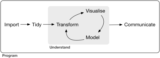
Every data science project involves importing, tidying, transforming, visualizing, modeling, and communicating data.

Import: Bring raw data into R.
Tidy: Reshape into a consistent format.
Transform: Create new variables and summaries.
Visualize: Explore patterns visually.
Model: Fit statistical or machine learning models.
Communicate: Share insights clearly.

Import: Bring raw data into R. (readxl)
Tidy: Reshape into a consistent format. (tidyr)
Transform: Create new variables and summaries. (dplyr)
Visualize: Explore patterns visually.
Model: Fit statistical or machine learning models.
Communicate: Share insights clearly.

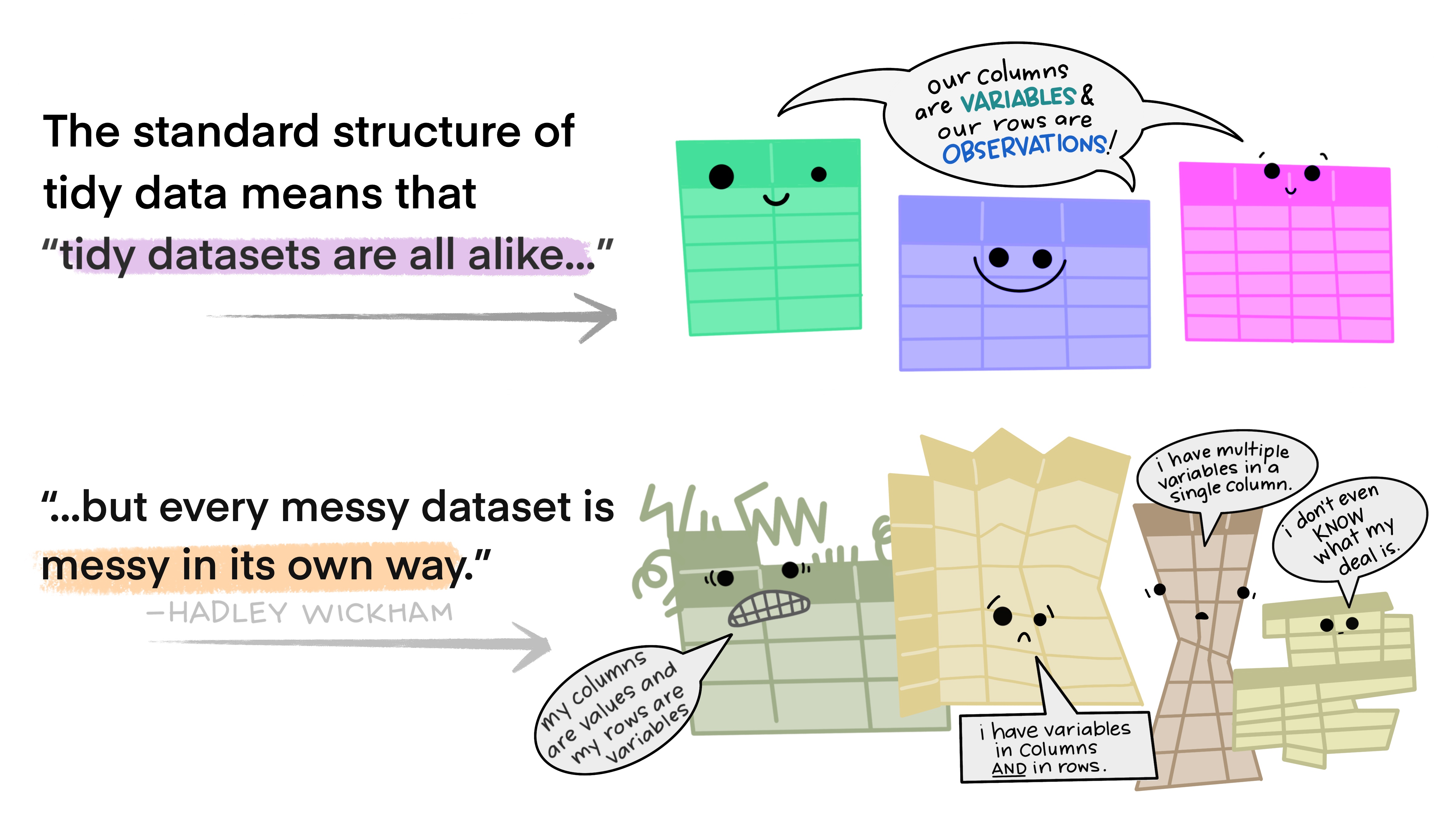
Why do we need tidy data?

“Tidy datasets are easy to manipulate, model, and visualize.” — Hadley Wickham

Tidy data make R tools work together smoothly.
Each tidy dataset is like a well-organized spreadsheet.
Making your data tidy allows you to avoid common errors that occurred in the data analysis.
The tidyr package has functions to make your data tidy.

Tidy Data

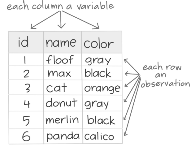
In tidy data:

Each variable is in a column
Each observation is in a row
Each cell is a single measurement.

https://openscapes.org/blog/2020-10-12-tidy-data/

Example 1

Consider four datasets with the same values of four variables country, year, population, and cases.

First, we have the tidy dataset version.

# A tibble: 6 × 4
  country      year  cases population
  <chr>       <dbl>  <dbl>      <dbl>
1 Afghanistan  1999    745   19987071
2 Afghanistan  2000   2666   20595360
3 Brazil       1999  37737  172006362
4 Brazil       2000  80488  174504898
5 China        1999 212258 1272915272
6 China        2000 213766 1280428583

tidy data because each variable is in a column , each observation is in a row, and each cell is a single measurement.

Consider another version:

# A tibble: 12 × 4
   country      year type            count
   <chr>       <dbl> <chr>           <dbl>
 1 Afghanistan  1999 cases             745
 2 Afghanistan  1999 population   19987071
 3 Afghanistan  2000 cases            2666
 4 Afghanistan  2000 population   20595360
 5 Brazil       1999 cases           37737
 6 Brazil       1999 population  172006362
 7 Brazil       2000 cases           80488
 8 Brazil       2000 population  174504898
 9 China        1999 cases          212258
10 China        1999 population 1272915272
11 China        2000 cases          213766
12 China        2000 population 1280428583

Not tidy because the last column is a summary statistic (count) of two variables.

Consider another version:

# A tibble: 6 × 3
  country      year rate             
  <chr>       <dbl> <chr>            
1 Afghanistan  1999 745/19987071     
2 Afghanistan  2000 2666/20595360    
3 Brazil       1999 37737/172006362  
4 Brazil       2000 80488/174504898  
5 China        1999 212258/1272915272
6 China        2000 213766/1280428583

Not tidy because the last column is a summary statistic (rate) of two variables, or there are two measurements involved in this column.

Consider one last version involving two datasets.

# A tibble: 3 × 3
  country     `1999` `2000`
  <chr>        <dbl>  <dbl>
1 Afghanistan    745   2666
2 Brazil       37737  80488
3 China       212258 213766

# A tibble: 3 × 3
  country         `1999`     `2000`
  <chr>            <dbl>      <dbl>
1 Afghanistan   19987071   20595360
2 Brazil       172006362  174504898
3 China       1272915272 1280428583

Not tidy data!

tidyr within the Tidyverse

The role of the tidyr package

tidyr works seamlessly with dplyr.
While dplyr focuses on data manipulation, tidyr focuses on data structure.
Together, they make your data clean and consistent before visualization or modeling.

tidyr’s comon functions

The tidyr provides functions for reshaping, organizing, and completing data.

Here, we will discuss the more common ones:

Purpose	Function 1	Function 2
Pivoting	`pivot_longer()`	`pivot_wider()`
Splitting / Combining	`separate()`	`unite()`

Example 2

Consider the data in the file “spotify.xlsx”. This dataset contains the global daily plays of the five most popular songs on the Spotify music streaming service in 2017.

Let’s read the dataset using the function read_excel() from the readxl library.

spotify_data = read_excel("spotify.xlsx")

Let’s preview the dataset.

spotify_data %>% head()

# A tibble: 6 × 7
  Date                  Day `Shape of You` Despacito `Something Just Like This`
  <dttm>              <dbl>          <dbl>     <dbl>                      <dbl>
1 2017-01-06 00:00:00     1       12287078        NA                         NA
2 2017-01-07 00:00:00     2       13190270        NA                         NA
3 2017-01-08 00:00:00     3       13099919        NA                         NA
4 2017-01-09 00:00:00     4       14506351        NA                         NA
5 2017-01-10 00:00:00     5       14275628        NA                         NA
6 2017-01-11 00:00:00     6       14372699        NA                         NA
# ℹ 2 more variables: HUMBLE. <dbl>, Unforgettable <dbl>

`pivot_longer()`

A common problem is a dataset where some of the column names are not names of variables, but values of a variable.

pivot_longer() transforms columns into rows (convert from wide to long format).

Let’s apply it to the spotify_data.

spotify_long = spotify_data %>% 
  pivot_longer(c(`Shape of You`, `Despacito`, `Something Just Like This`, 
                 `HUMBLE.`, `Unforgettable`), 
               names_to = "Song", 
               values_to = "Plays")

Remark on variable names

In R, variable names (column names) typically:

Cannot contain spaces or special symbols like “-”, “/”, or “%”.
Cannot start with a number.

So, when a dataset has column names like “Shape of You” or “Something Just Like This”, R cannot recognize them directly unless you enclose them in backticks (“`”).

There are some exceptions though, like when you first define the name of the variable like “Song”.

The long version of the data

A Song column with the names of the songs in the dataset.
A Plays column with the number of plays of each song for each date.

spotify_long %>% head()

# A tibble: 6 × 4
  Date                  Day Song                        Plays
  <dttm>              <dbl> <chr>                       <dbl>
1 2017-01-06 00:00:00     1 Shape of You             12287078
2 2017-01-06 00:00:00     1 Despacito                      NA
3 2017-01-06 00:00:00     1 Something Just Like This       NA
4 2017-01-06 00:00:00     1 HUMBLE.                        NA
5 2017-01-06 00:00:00     1 Unforgettable                  NA
6 2017-01-07 00:00:00     2 Shape of You             13190270

`pivot_wider()`

pivot_wider() is the opposite of pivot_longer(). We use it when an observation is scattered across multiple rows.

spotify_wide = spotify_long %>% 
  pivot_wider(names_from = "Song", values_from = "Plays")
spotify_wide %>% head()

# A tibble: 6 × 7
  Date                  Day `Shape of You` Despacito `Something Just Like This`
  <dttm>              <dbl>          <dbl>     <dbl>                      <dbl>
1 2017-01-06 00:00:00     1       12287078        NA                         NA
2 2017-01-07 00:00:00     2       13190270        NA                         NA
3 2017-01-08 00:00:00     3       13099919        NA                         NA
4 2017-01-09 00:00:00     4       14506351        NA                         NA
5 2017-01-10 00:00:00     5       14275628        NA                         NA
6 2017-01-11 00:00:00     6       14372699        NA                         NA
# ℹ 2 more variables: HUMBLE. <dbl>, Unforgettable <dbl>

We can also apply it to the table2 dataset in the previous section.

table2

# A tibble: 12 × 4
   country      year type            count
   <chr>       <dbl> <chr>           <dbl>
 1 Afghanistan  1999 cases             745
 2 Afghanistan  1999 population   19987071
 3 Afghanistan  2000 cases            2666
 4 Afghanistan  2000 population   20595360
 5 Brazil       1999 cases           37737
 6 Brazil       1999 population  172006362
 7 Brazil       2000 cases           80488
 8 Brazil       2000 population  174504898
 9 China        1999 cases          212258
10 China        1999 population 1272915272
11 China        2000 cases          213766
12 China        2000 population 1280428583

The wider version of table2 is:

table2 %>%
    pivot_wider(names_from = type, values_from = count)

# A tibble: 6 × 4
  country      year  cases population
  <chr>       <dbl>  <dbl>      <dbl>
1 Afghanistan  1999    745   19987071
2 Afghanistan  2000   2666   20595360
3 Brazil       1999  37737  172006362
4 Brazil       2000  80488  174504898
5 China        1999 212258 1272915272
6 China        2000 213766 1280428583

Example 3

Consider an industrial engineer who receives a messy Excel file from a manufacturing client. The data file is called “industrial_dataset.xlsx”, which file includes data about machine maintenance logs, production output, and operator comments.

industrial_data = read_excel("industrial_dataset.xlsx")

We use this dataset to illustrate the functions separate() and unite().

Let’s preview the data.

industrial_data %>% head()

# A tibble: 6 × 5
  `Machine ID` `Output (units)` `Maintenance Date`  Operator Comment            
         <dbl> <chr>            <dttm>              <chr>    <chr>              
1          101 1200             2023-01-10 00:00:00 Ana      "ok"               
2          101 1200             2023-01-10 00:00:00 Ana      "ok"               
3          102 1050             2023-01-12 00:00:00 Bob      "Needs oil!"       
4          103 error            2023-01-13 00:00:00 Charlie  "All good\r\n"     
5          103 950              2023-01-13 00:00:00 Charlie  "All good\r\n"     
6          104 900              2023-01-14 00:00:00 <NA>     "Delay: power issu…

`separate()`

separate() pulls apart one column into multiple columns, by splitting wherever a separator character appears.

Consider the column Comment from industrial_data.

industrial_data %>% select(Comment)

# A tibble: 100 × 1
   Comment               
   <chr>                 
 1 "ok"                  
 2 "ok"                  
 3 "Needs oil!"          
 4 "All good\r\n"        
 5 "All good\r\n"        
 6 "Delay: power issue"  
 7 "completed"           
 8 "completed"           
 9 "All good\r\n"        
10 "Requires part: valve"
# ℹ 90 more rows

The column has some values such as “Requires part: valve” and “Delay: maintenance” that we may want to split into columns.

# A tibble: 100 × 1
   Comment               
   <chr>                 
 1 "ok"                  
 2 "ok"                  
 3 "Needs oil!"          
 4 "All good\r\n"        
 5 "All good\r\n"        
 6 "Delay: power issue"  
 7 "completed"           
 8 "completed"           
 9 "All good\r\n"        
10 "Requires part: valve"
# ℹ 90 more rows

Using separate(), we split the values in the column according to the colon “:”.

augmented_data = industrial_data  %>% 
separate(Comment, into = c("First_comment", "Second_comment"), 
         sep = ":")

The result is two columns.

augmented_data %>% select(`First_comment`, `Second_comment`) %>%  head()

# A tibble: 6 × 2
  First_comment  Second_comment
  <chr>          <chr>         
1 "ok"            <NA>         
2 "ok"            <NA>         
3 "Needs oil!"    <NA>         
4 "All good\r\n"  <NA>         
5 "All good\r\n"  <NA>         
6 "Delay"        " power issue"

`unite()`

unite() is the inverse of separate(). It combines multiple columns into a single column.

augmented_data  %>% 
  unite(Comment, First_comment, Second_comment, sep = ": ") %>% 
    select(Comment)

In the unite() function, the first input is the name of the new column, the other inputs are the columns to be united.

The result.

augmented_data  %>% 
  unite(Comment, First_comment, Second_comment, sep = ": ") %>% 
    select(Comment)

# A tibble: 100 × 1
   Comment                
   <chr>                  
 1 "ok: NA"               
 2 "ok: NA"               
 3 "Needs oil!: NA"       
 4 "All good\r\n: NA"     
 5 "All good\r\n: NA"     
 6 "Delay:  power issue"  
 7 "completed: NA"        
 8 "completed: NA"        
 9 "All good\r\n: NA"     
10 "Requires part:  valve"
# ℹ 90 more rows

Data Wrangling

Data wrangling is the process of transforming raw data into a clean and structured format.
It involves merging, reshaping, filtering, and organizing data for analysis.
Here, we illustrate some special functions of the tidyverse for cleaning common issues with a dataset.

Add an index column

In some cases, it is useful to have a unique identifier for each row in the dataset. We can create an identifier using the functions mutate() and row_number() with some extra syntaxis.

industrial_data_single = industrial_data %>% 
                         mutate(ID = row_number())

The new column is appended to the end of the dataframe.

industrial_data_single %>%  head()

# A tibble: 6 × 6
  `Machine ID` `Output (units)` `Maintenance Date`  Operator Comment          ID
         <dbl> <chr>            <dttm>              <chr>    <chr>         <int>
1          101 1200             2023-01-10 00:00:00 Ana      "ok"              1
2          101 1200             2023-01-10 00:00:00 Ana      "ok"              2
3          102 1050             2023-01-12 00:00:00 Bob      "Needs oil!"      3
4          103 error            2023-01-13 00:00:00 Charlie  "All good\r\…     4
5          103 950              2023-01-13 00:00:00 Charlie  "All good\r\…     5
6          104 900              2023-01-14 00:00:00 <NA>     "Delay: powe…     6

To bring it to the beginning of the array, we can use the select() and everything() functions.

industrial_data_single = industrial_data_single %>% 
select(ID, everything())

industrial_data_single %>%  head()

# A tibble: 6 × 6
     ID `Machine ID` `Output (units)` `Maintenance Date`  Operator Comment      
  <int>        <dbl> <chr>            <dttm>              <chr>    <chr>        
1     1          101 1200             2023-01-10 00:00:00 Ana      "ok"         
2     2          101 1200             2023-01-10 00:00:00 Ana      "ok"         
3     3          102 1050             2023-01-12 00:00:00 Bob      "Needs oil!" 
4     4          103 error            2023-01-13 00:00:00 Charlie  "All good\r\…
5     5          103 950              2023-01-13 00:00:00 Charlie  "All good\r\…
6     6          104 900              2023-01-14 00:00:00 <NA>     "Delay: powe…

Fill blank cells

In the industrial_data_single, there are columns with missing values. We can fill them with specific values or text using replace_na() function. In this function, we use the syntaxis 'Variable' = 'Replace', where the Variable is the column in the dataset and Replace is the text or number to fill the entry in.

Let’s fill in the missing entries of the columns Operator, Maintenance Date, and Comment.

complete_data = industrial_data_single %>% 
                  replace_na( list(
                  Operator = "Unknown",
                  `Maintenance Date` = as.Date("2023-01-01"),
                  Comment = "None") 
                  )

complete_data %>%  head()

# A tibble: 6 × 6
     ID `Machine ID` `Output (units)` `Maintenance Date`  Operator Comment      
  <int>        <dbl> <chr>            <dttm>              <chr>    <chr>        
1     1          101 1200             2023-01-10 00:00:00 Ana      "ok"         
2     2          101 1200             2023-01-10 00:00:00 Ana      "ok"         
3     3          102 1050             2023-01-12 00:00:00 Bob      "Needs oil!" 
4     4          103 error            2023-01-13 00:00:00 Charlie  "All good\r\…
5     5          103 950              2023-01-13 00:00:00 Charlie  "All good\r\…
6     6          104 900              2023-01-14 00:00:00 Unknown  "Delay: powe…

Replace values

There are some cases in which columns have some undesired or unwatned values. Consider the Output (units) as an example.

complete_data %>% select(`Output (units)`) %>% head()

# A tibble: 6 × 1
  `Output (units)`
  <chr>           
1 1200            
2 1200            
3 1050            
4 error           
5 950             
6 900

The column has the numbers of units but also text such as “error”.

We can replace the “error” in this column by a user-specified value, say, 0. To this end, we use the functions mutate() and na_if().

complete_data = complete_data %>% 
mutate(`Output (units)` = na_if(`Output (units)`, "error"))

# Let's check the column.
complete_data %>%  select(`Output (units)`) %>%  head()

# A tibble: 6 × 1
  `Output (units)`
  <chr>           
1 1200            
2 1200            
3 1050            
4 <NA>            
5 950             
6 900

However, the new column is character (chr)!

We turn the column numeric using the functions mutate() and as.numeric().

complete_data = complete_data %>% 
mutate(`Output (units)` = as.numeric(`Output (units)`))

complete_data %>%  select(`Output (units)`) %>%  head()

# A tibble: 6 × 1
  `Output (units)`
             <dbl>
1             1200
2             1200
3             1050
4               NA
5              950
6              900

Now, the column is numeric or dbl!

A new library: stringr

stringr provides a consistent set of functions for working with strings.
It is also part of the tidyverse collection.
https://stringr.tidyverse.org/

Load it to Google Colab with the following code.

library(stringr)

Example 3 (cont.)

Let’s reconsider the Example 4 after splitting the column Comment into two columns First_Comment and Second_comment.

augmented_data

# A tibble: 100 × 6
   `Machine ID` `Output (units)` `Maintenance Date`  Operator First_comment  
          <dbl> <chr>            <dttm>              <chr>    <chr>          
 1          101 1200             2023-01-10 00:00:00 Ana      "ok"           
 2          101 1200             2023-01-10 00:00:00 Ana      "ok"           
 3          102 1050             2023-01-12 00:00:00 Bob      "Needs oil!"   
 4          103 error            2023-01-13 00:00:00 Charlie  "All good\r\n" 
 5          103 950              2023-01-13 00:00:00 Charlie  "All good\r\n" 
 6          104 900              2023-01-14 00:00:00 <NA>     "Delay"        
 7          105 870              NA                  DAVE     "completed"    
 8          105 800              2023-01-21 00:00:00 dave     "completed"    
 9          102 870              2023-01-25 00:00:00 Charlie  "All good\r\n" 
10          102 800              2023-01-20 00:00:00 Charlie  "Requires part"
# ℹ 90 more rows
# ℹ 1 more variable: Second_comment <chr>

Remove characters

Something that we notice is that the column First_Comment has some extra characters like “\n” that may be useless when working with the data.

We can remove them using the function str_trim() from the stringr package.

augmented_data = augmented_data  %>% 
mutate(First_comment = str_trim(First_comment, side = "both"))

Let’s see the cleaned column.

augmented_data %>%  select(`First_comment`)

# A tibble: 100 × 1
   First_comment
   <chr>        
 1 ok           
 2 ok           
 3 Needs oil!   
 4 All good     
 5 All good     
 6 Delay        
 7 completed    
 8 completed    
 9 All good     
10 Requires part
# ℹ 90 more rows

We can remove special characters such as “!” from all cells in the column.

To do this, we use the functions mutate() and str_remove_all() with the character to remove. That is, we create a new cleaned variable without the specific character.

augmented_data %>%  
  mutate("First_comment" = str_remove_all(`First_comment`, "!")) %>% 
  select(`First_comment`) %>% head()

# A tibble: 6 × 1
  First_comment
  <chr>        
1 ok           
2 ok           
3 Needs oil    
4 All good     
5 All good     
6 Delay

Transform text case

When working with text columns containing names, we may have different ways of writing. A common case is when having lower case or upper case names or a combination thereof.

For example, consider the column Operator containing the names of the operators.

complete_data %>% select(Operator) %>%  head()

# A tibble: 6 × 1
  Operator
  <chr>   
1 Ana     
2 Ana     
3 Bob     
4 Charlie 
5 Charlie 
6 Unknown

Remove extra spaces

To deal with names, we first use the str_trim() to remove leading and trailing characters from strings.

complete_data =  complete_data %>% 
mutate(Operator = str_trim(Operator))

complete_data %>% select(Operator) %>%  head()

# A tibble: 6 × 1
  Operator
  <chr>   
1 Ana     
2 Ana     
3 Bob     
4 Charlie 
5 Charlie 
6 Unknown

Change to lowercase letters

We can turn all names to lowercase using the function str_to_lower().

complete_data %>% 
mutate(Operator = str_to_lower(Operator)) %>% 
select(Operator) %>% 
head()

# A tibble: 6 × 1
  Operator
  <chr>   
1 ana     
2 ana     
3 bob     
4 charlie 
5 charlie 
6 unknown

Change to uppercase letters

We can turn all names to uppercase using the function str_to_upper().

complete_data %>% 
mutate(Operator = str_to_upper(Operator)) %>% 
select(Operator) %>% 
head()

# A tibble: 6 × 1
  Operator
  <chr>   
1 ANA     
2 ANA     
3 BOB     
4 CHARLIE 
5 CHARLIE 
6 UNKNOWN

Capitalize the first letter

We can convert all names to title case using the function str_to_title().

complete_data %>% 
mutate(Operator = str_to_title(Operator)) %>% 
select(Operator) %>% 
head()

# A tibble: 6 × 1
  Operator
  <chr>   
1 Ana     
2 Ana     
3 Bob     
4 Charlie 
5 Charlie 
6 Unknown

More on tidyr and stringr

https://r4ds.hadley.nz/

Tidy Data

Agenda

Load the libraries

Tidy Data

A new library: tidyr

Data science workflow

Why do we need tidy data?

Tidy Data

Example 1

tidyr within the Tidyverse

The role of the tidyr package

tidyr’s comon functions

Example 2

pivot_longer()

Remark on variable names

The long version of the data

pivot_wider()

Example 3

Let’s preview the data.

separate()

unite()

Data Wrangling

Data Wrangling

Add an index column

Fill blank cells

Replace values

A new library: stringr

Example 3 (cont.)

Remove characters

Transform text case

Remove extra spaces

Change to lowercase letters

Change to uppercase letters

Capitalize the first letter

More on tidyr and stringr

Return to main page

`pivot_longer()`

`pivot_wider()`

`separate()`

`unite()`