Types of Variables and Univariate Plots

IN2039: Data Visualization for Decision Making

Alan R. Vazquez

Department of Industrial Engineering

Agenda

1. Types of Variables
2. One Categorical Variable
3. One Numerical Variable

Types of variables

Before creating a graph, we must examine the type of values that our dataset variables take.

There are two main types of variables:

• Numerical variables.

• Categorical variables.

Numerical variables

These take values that represent numerical measurements or quantities.

• Height (in centimeters).
• Weight (in kilograms).
• Age (in years).
• Price (in dollars).
• Time (in hours or seconds).
• Exam score (number of points on a 100-point scale).

Types of numerical variables

Numerical variables are divided into two types:

• Discrete: variables that take integer values.

Examples:

1. Number of children (0, 1, 2, or 3)
2. Number of students in a class (20, 30, or 35)
3. Number of books in a library (10,000, 15,000, 20,000)

• Continuous: variables that have a large range of possible values.

Examples:

1. A person’s height (could be within the range of 1.60 m to 1.85 m)
2. Ambient temperature (could be within the range of -30 \(^\circ\)C to 50 \(^\circ\)C)
3. Time for an Uber to arrive (between 5 and 60 minutes)

Categorical variables

These take values that fall into categories.

A category is a class or division of people or things that share particular characteristics.

Variable	Categories
Amazon review	1\(\bigstar\), 2\(\bigstar\), 3\(\bigstar\), 4\(\bigstar\), 5\(\bigstar\)
Country of origin	México, Canadá, EUA
Postal code	72703, 90034, 3000, …

Classification of categorical variables

Categorical variables are divided into two important types:

• Nominal
• Ordinal

The distinction depends on whether the categories have a meaningful order or not.

Nominal categorical variables

A categorical variable is nominal if its categories do not have a specific order.

Examples:

• Political party affiliation (Democrat or Republican).
• Dog breed (Shepherd, Hound, Terrier, Other).
• Computer operating system (Windows, macOS, Linux).

Ordinal categorical variables

A categorical variable is ordinal if its categories do have a meaningful order.

Examples:

• T-shirt size (Small, Medium, Large).
• Education level (High School, University, Postgraduate).
• Income level (Less than $250K, $250K-$500K, More than $500K)

It is important to note that with an ordinal variable, the difference between, say, small and medium is not necessarily the same as the difference between medium and large. Additionally, the differences between consecutive categories may not be quantifiable. Think about star ratings in a restaurant review—how much better is one star compared to two stars?

Interesting fact…

Integer values (e.g., 1, 2, 3, …, 5) can represent nominal or ordinal categorical variables.

Representation	1	2	3	4
Blood Type	A	B	AB	O
Review	Bad	Fair	Good	Very Good

In practice, boolean values (TRUE and FALSE) often represent nominal categories.

Remember

A general difference is …

• Quantitative variables (discrete or continuous) are those where addition or subtraction makes sense.

• Categorical variables (nominal or ordinal) are those where addition or subtraction does NOT make sense.

One Categorical Variable

Example 1: Penguins dataset

We will illustrate the concepts using the penguins.xlsx dataset. We will focus on visualizing the categorical variable species.

library(readxl)
library(tidyverse)
library(writexl)
penguins_data = read_excel("penguins.xlsx")
penguins_data %>% 
  select(species, island, sex) %>%
  head()

# A tibble: 6 × 3
  species island    sex   
  <chr>   <chr>     <chr> 
1 Adelie  Torgersen male  
2 Adelie  Torgersen female
3 Adelie  Torgersen female
4 Adelie  Torgersen <NA>  
5 Adelie  Torgersen female
6 Adelie  Torgersen male  

Principle 2: Turn data into information

As a starting point,we compute the frequencies of each category of species using the dplyr functions group_by(), summarise(), and n().

• The group_by() function takes an existing table and converts it into a grouped table where operations are performed “by group”.

• The n() function counts the values in a category.

frequencies_species = penguins_data %>% 
                      group_by(species) %>% 
                      summarise("Frequency" = n())

Frequency table

frequencies_species

# A tibble: 3 × 2
  species   Frequency
  <chr>         <int>
1 Adelie          152
2 Chinstrap        68
3 Gentoo          124

We save the frequency table for further processing with Flourish studio using the command below.

# write_xlsx(frequencies_species, "PenguinsDataFlourish.xlsx")

Bar chart

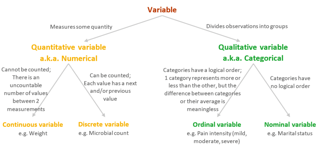
Shows frequencies of the categories of a categorical variable.

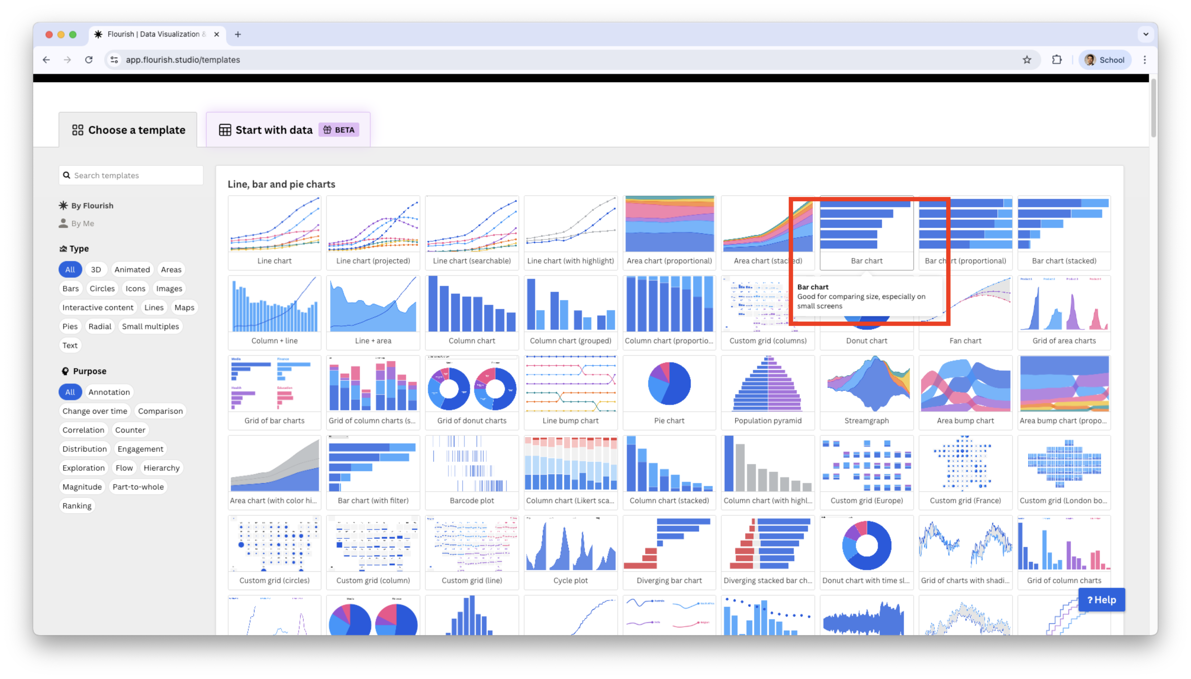
Construct a bar chart in Flourish

In the visualization gallery, choose Bar Chart.

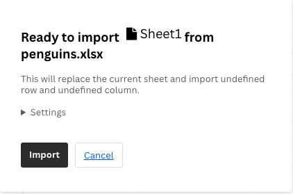
Replace the data with your own

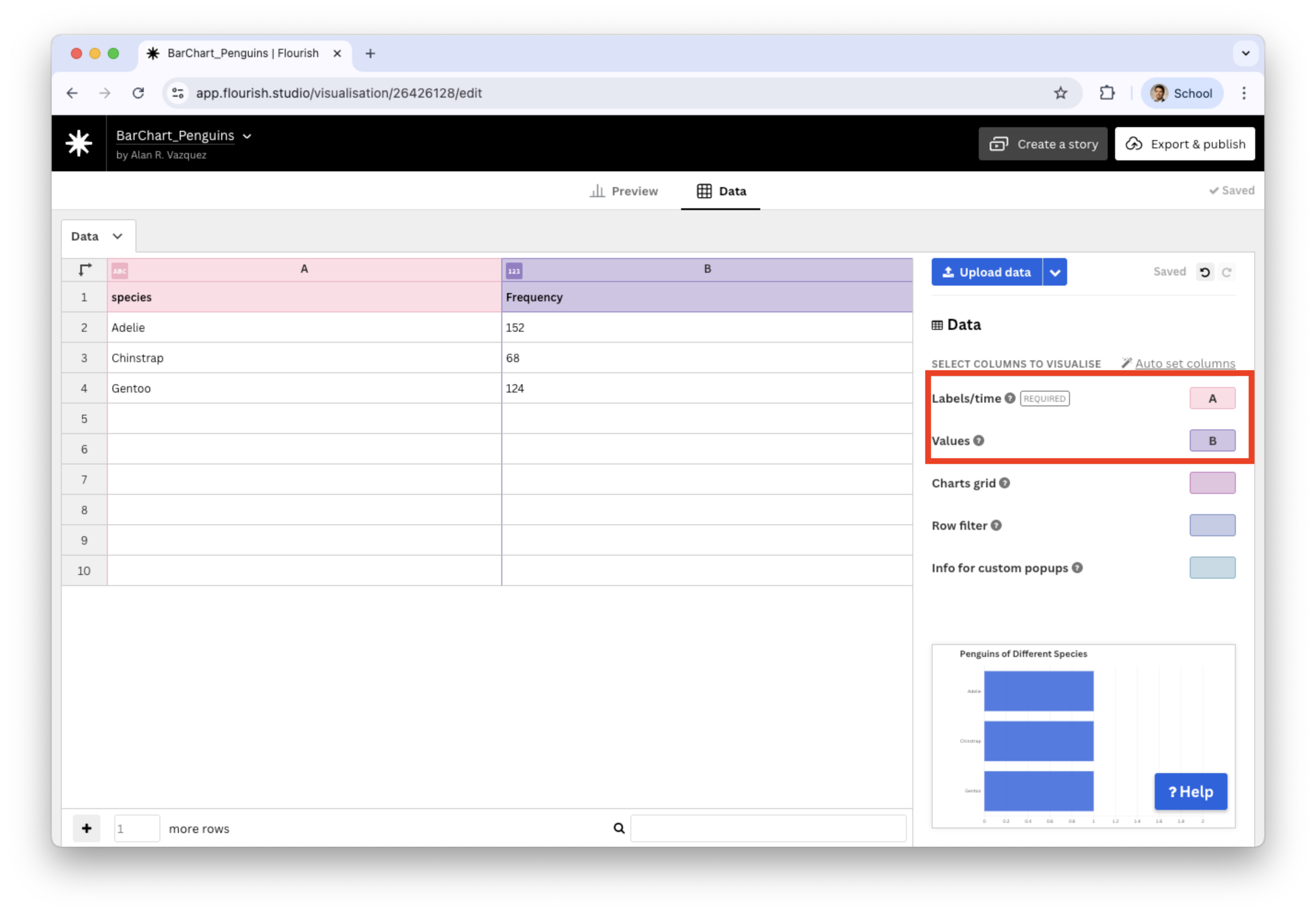
Select the correct variables

Make sure that you uploaded the file “PenguinsDataFlourish.xlsx” and not the original one.

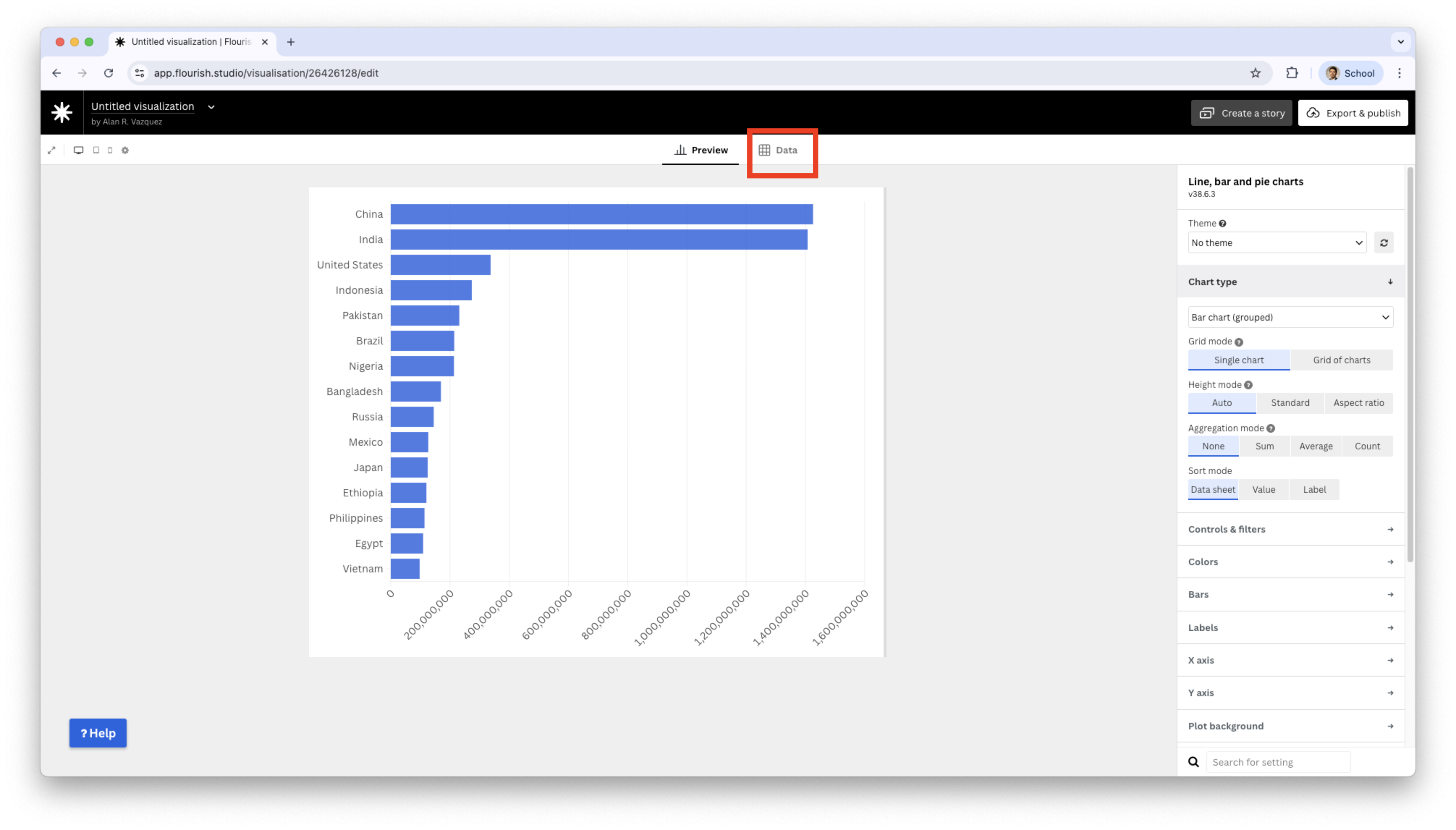
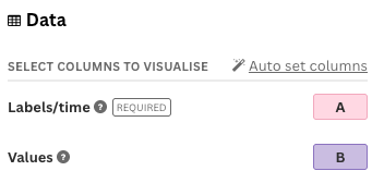
Now, we assign the variable species to Labels/time, and Frequency to Values.

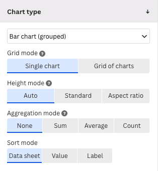
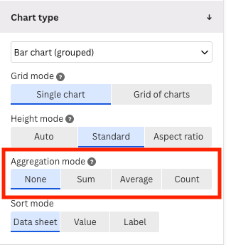
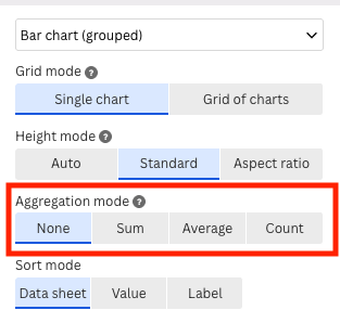
The preview plot has all bars at the same height. To replace the height for the frequencies of the categories, we change the Agregation mode to None.

We also change the Height mode to Standard to enhance the visualization.

Principle 1: Define the message

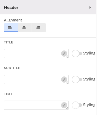
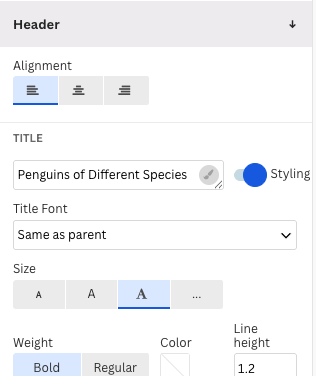
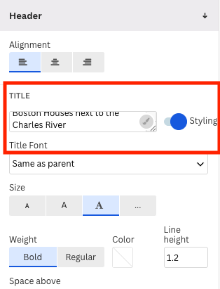
Following Principle 1 of data visualization, we add a header or title to the plot by going to the section Header.

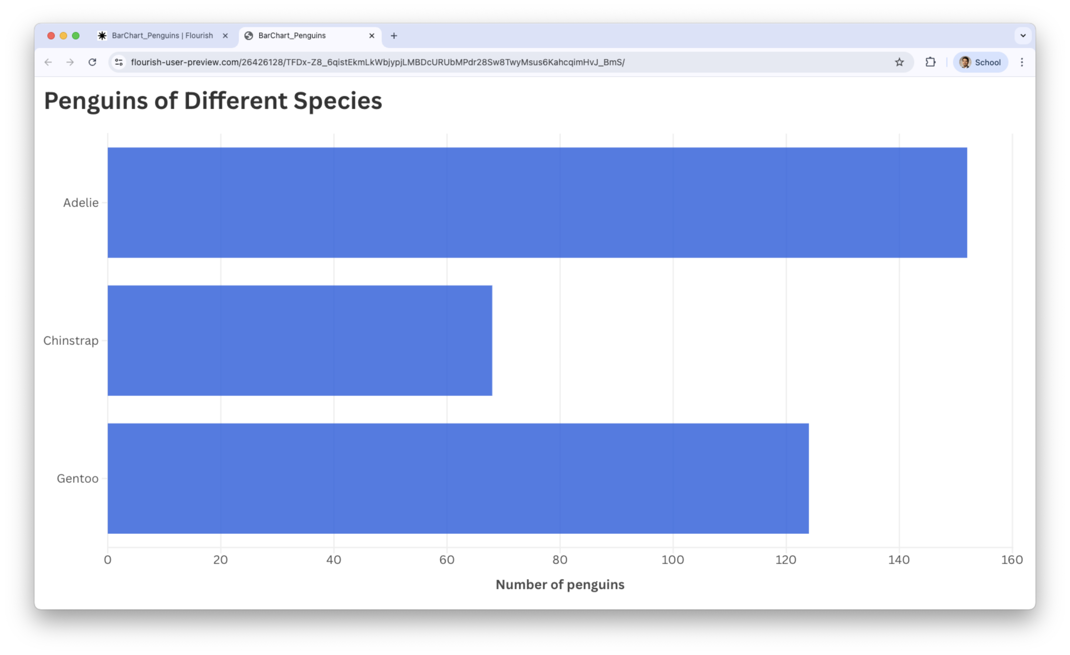
Final bar chart

We see that most penguins are Adelie.

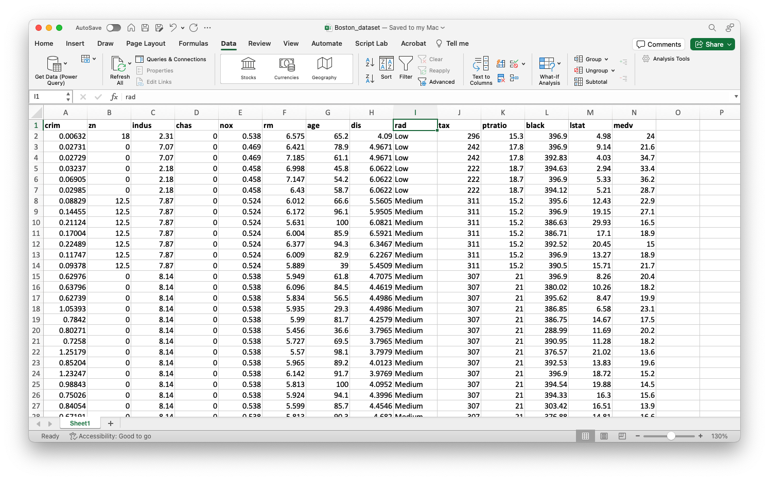
Example 2: Boston Housing Dataset

This dataset contains information collected by the U.S. Census Bureau on housing in the Boston, Massachusetts area. The dataset is in Boston_dataset.xlsx.

We concentrate on the following variables:

• chas : Whether the house is next to the Charles River (1: Yes and 0: No)

• rad : Index of accessibility to radial highways (0: Low, 1: Medium, 2: High).

Data wrangling with R

To create a effective bar plots in Flourish, we must wrangle the variables chas and rad a little bit.

Specifically, we must ensure that these variables are categorical and their categories have the appropriate names.

Boston_dataset = read_excel("Boston_dataset.xlsx")
Boston_dataset %>% select(`chas`, `rad`) %>%  head()

# A tibble: 6 × 2
   chas   rad
  <dbl> <dbl>
1     0     0
2     0     0
3     0     0
4     0     0
5     0     0
6     0     0

The variables are numeric because their header shows a dbl.

# A tibble: 6 × 2
   chas   rad
  <dbl> <dbl>
1     0     0
2     0     0
3     0     0
4     0     0
5     0     0
6     0     0

To set variables as categorical we use the functions mutate() and as.factor().

Boston_dataset_wr = Boston_dataset %>% 
                    mutate(`chas` = as.factor(`chas`)) %>% 
                    mutate(`rad` = as.factor(`rad`))

Now the header of the variables show a fct indicating that the variables are categorical.

Boston_dataset_wr  %>% select(`chas`, `rad`) 

# A tibble: 506 × 2
   chas  rad  
   <fct> <fct>
 1 0     0    
 2 0     0    
 3 0     0    
 4 0     0    
 5 0     0    
 6 0     0    
 7 0     1    
 8 0     1    
 9 0     1    
10 0     1    
# ℹ 496 more rows

Next, we replace the 0 and 1 of chas for the label “No” and “Yes”, respectively. To this end, we use the function mutate() and caste_match().

Boston_dataset_wr = Boston_dataset_wr %>% 
  mutate(`chas` = case_match(`chas`, "0" ~ "No", "1" ~ "Yes"))

Using the same functions, we replace the 0, 1, and 2 in the variable rad by “Low”, “Medium”, and “High”, respectively.

Boston_dataset_wr = Boston_dataset_wr %>% 
  mutate(`rad` = case_match(`rad`, "0" ~ "Low", "1" ~ "Medium",
                            "2" ~ "High"))

Now, the columns show the actual category labels instead of the coded (or number) labels.

Boston_dataset_wr  %>% select(`chas`, `rad`) 

# A tibble: 506 × 2
   chas  rad   
   <chr> <chr> 
 1 No    Low   
 2 No    Low   
 3 No    Low   
 4 No    Low   
 5 No    Low   
 6 No    Low   
 7 No    Medium
 8 No    Medium
 9 No    Medium
10 No    Medium
# ℹ 496 more rows

For the bar chart, we compute the frequencies of the categories of chas and rad.

frequencies_Boston_chas = Boston_dataset_wr %>% 
                      group_by(`chas`) %>% 
                      summarise("Frequency" = n())

frequencies_Boston_rad = Boston_dataset_wr %>% 
                      group_by(`rad`) %>% 
                      summarise("Frequency" = n())

We save the new datasets using the function write_xlsx() from the writexl package in R.

#write_xlsx(frequencies_Boston_chas, "BostonDataFlourishChas.xlsx")
#write_xlsx(frequencies_Boston_rad, "BostonDataFlourishRad.xlsx")

We then proceed to visualize the processed data using Flourish.

Let’s create a bar chart for chas.

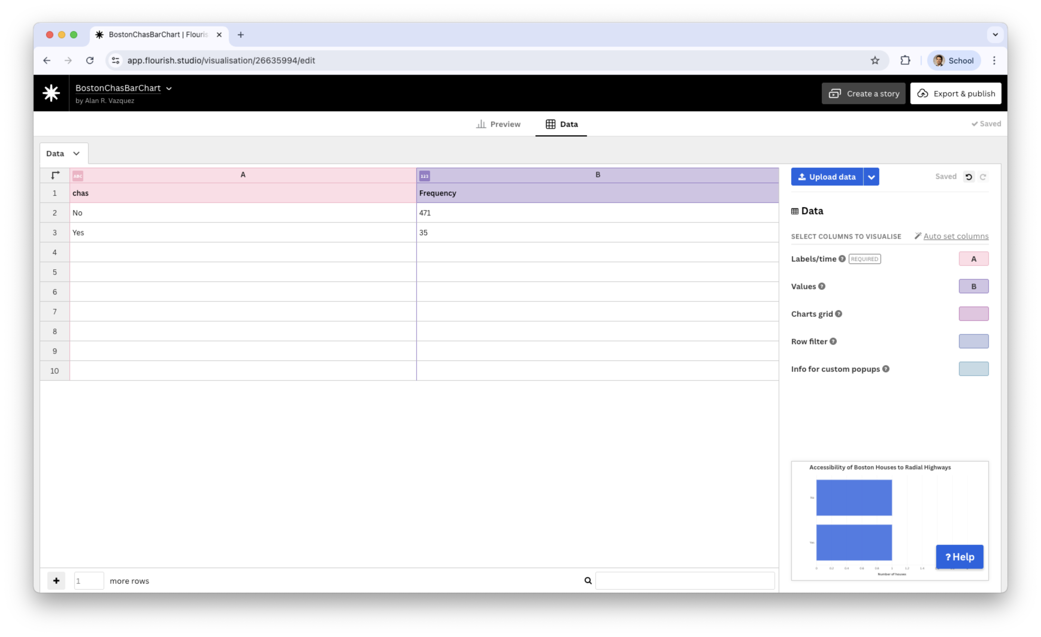
We load the dataset “BostonDataFlourishChas.xlsx” into Flourish.

We assign the chas variable to the Labels/time and Frequency to Values.

Now, we go back to the Preview tab and set Aggregation mode to None.

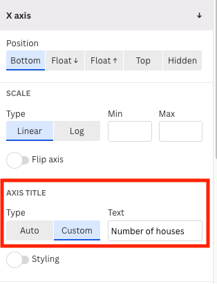
In the menu of the Preview tab, we add a title and a good label for the horizontal axis.

Bar chart for chas

Similarly, we create a bar chart for rad

Collapsing categories

Some categorical variables tend to have many categories. For example, states in a country or postal codes. In these cases, it can be difficult to visualize all the categories in a single graph.

One strategy for developing an effective visualization is to collapse categories.

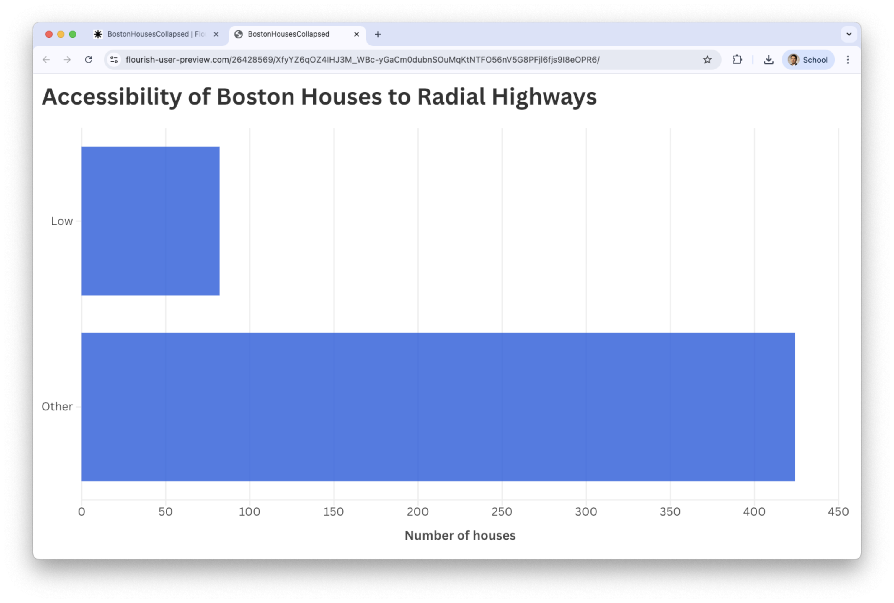
For example, in the variable rad, we can collapse the categories Medium and High into a single category called Other.

We collapse categories using the function called case_when().

Boston_dataset_simple = Boston_dataset_wr %>% 
      mutate(rad = case_when(rad != "Low" ~ "Other",
                             rad == "Low" ~ "Low"))

Collapsing categories simplifies the graph and allows us to emphasize a category like Low and see how it compares to the other categories (as a whole).

We save the new dataset using the function write_xlsx().

# write_xlsx(Boston_dataset_simple, "BostonCollapsed.xlsx")

We then proceed to visualize the processed data using Flourish.

The resulting bar chart

One Numerical Variable

Example 3

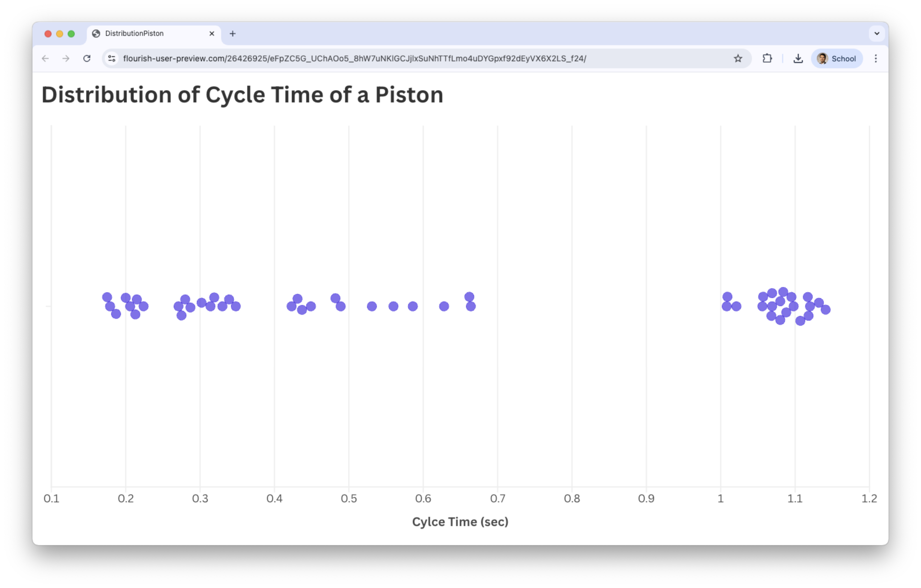
A piston is a mechanical device found in most engines.

One measure of a piston’s performance is the time it takes to complete a cycle, which we call “cycle time” and is measured in seconds.

The file “CYLT.xlsx” contains 50 cycle times of a piston operating under fixed conditions.

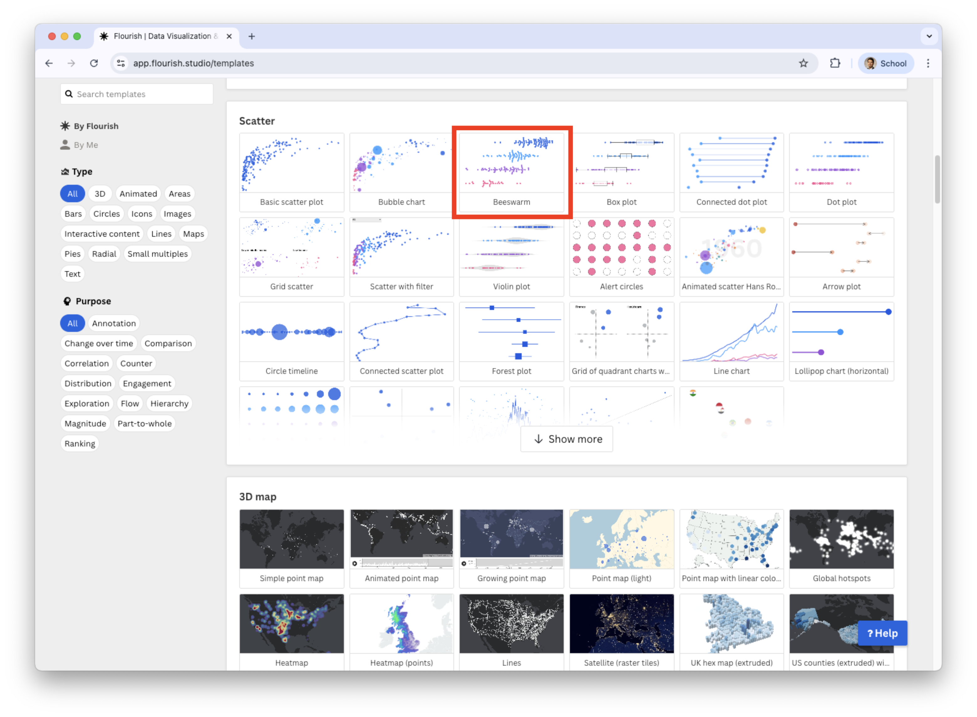
Beeswarm

Visualizes the distribution of individual observations along a numeric axis.

• Each point represents one data value, and the points are arranged to avoid overlapping—similar to bees clustering around a hive.
• This makes it easy to see where observations are dense or sparse, while still showing every individual data point.

• Unlike histograms, which aggregate counts into bars, beeswarm plots preserve every point, giving a more detailed picture of the underlying distribution.

Beeswarm in Flourish

Beeswarm is in the section Scatter of the catalog of visualizations in Flourish.

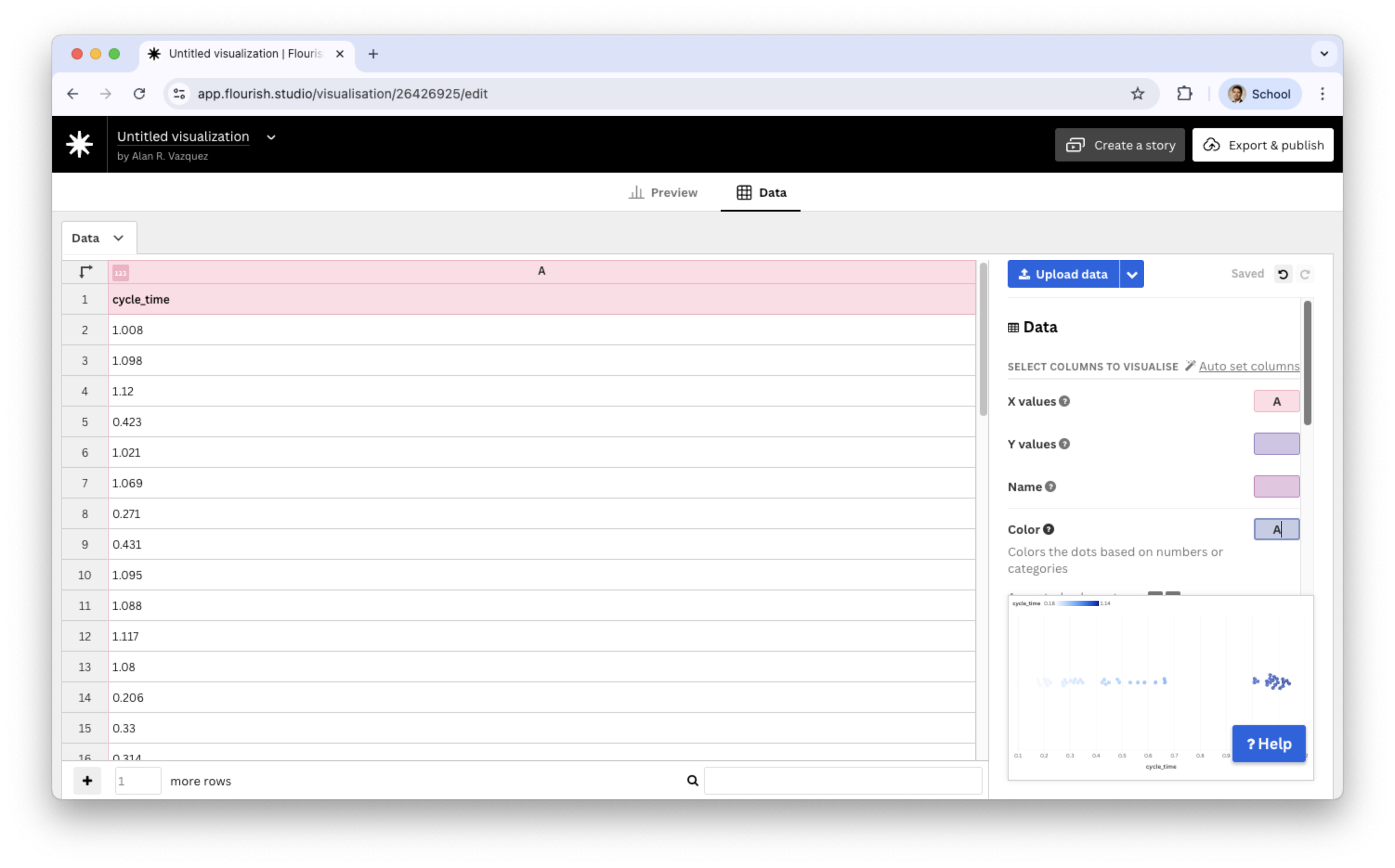
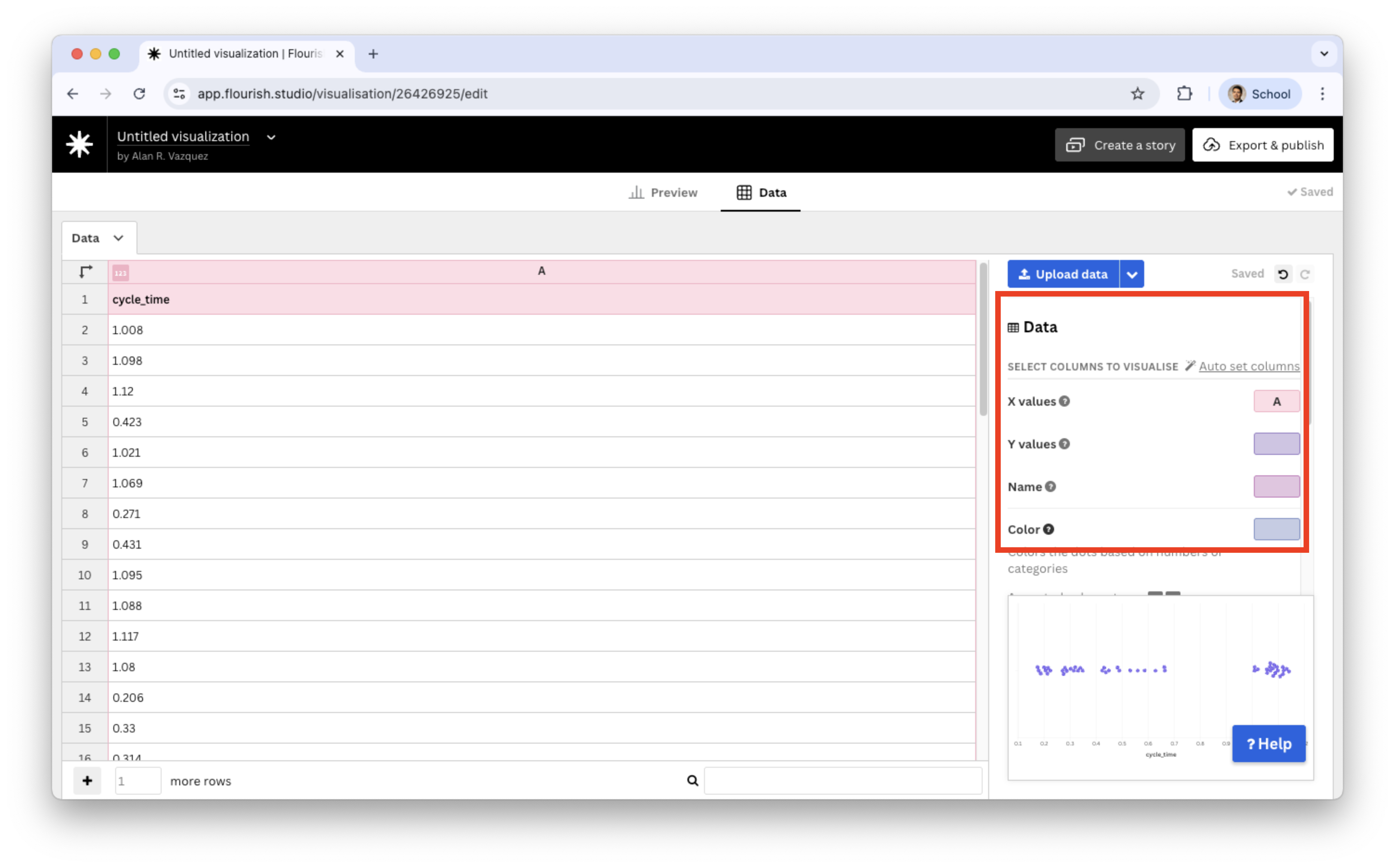
In the Beeswarm plot, we replace the current data with the data in “CYLT.xlsx” in the Data tab.

In the Data tab, we only assign the cycle_time variable to the X values section.

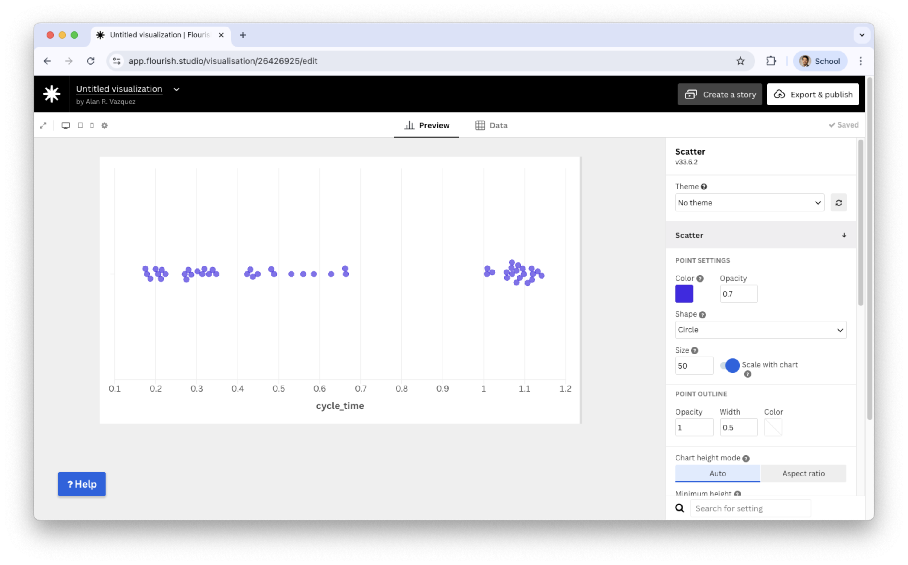
Let’s go back to the Preview tab.

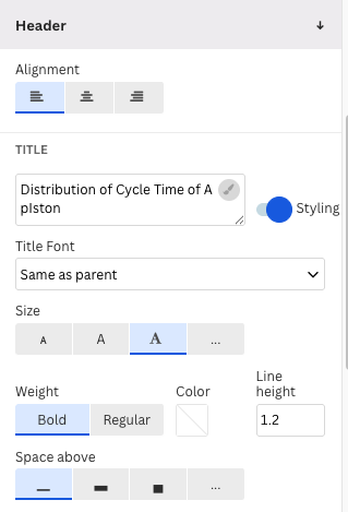
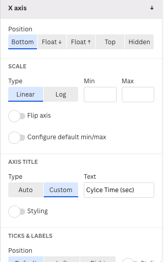
There, we modify the label of the horizontal axis X and header in the sections X axis and Header.

Beeswarm plot

What to look for in a beeswarm plot?

• Clusters of points that reveal dense regions in the distribution.
• Areas where points are more spread out, indicating low-frequency regions.
• Gaps along the axis where no observations appear.
• Outliers, visible as isolated points far from the main cluster.
• The overall shape of the distribution formed by the pattern of points.

Return to main page