import pandas as pd
import matplotlib.pyplot as plt
import seaborn as sns
from sklearn.model_selection import train_test_split, GridSearchCV
from sklearn.tree import DecisionTreeClassifier, plot_tree
from sklearn.preprocessing import StandardScaler
from sklearn.metrics import confusion_matrix, ConfusionMatrixDisplay
from sklearn.metrics import accuracy_score, recall_score, precision_scoreClassification Trees
IN5148: Statistics and Data Science with Applications in Engineering
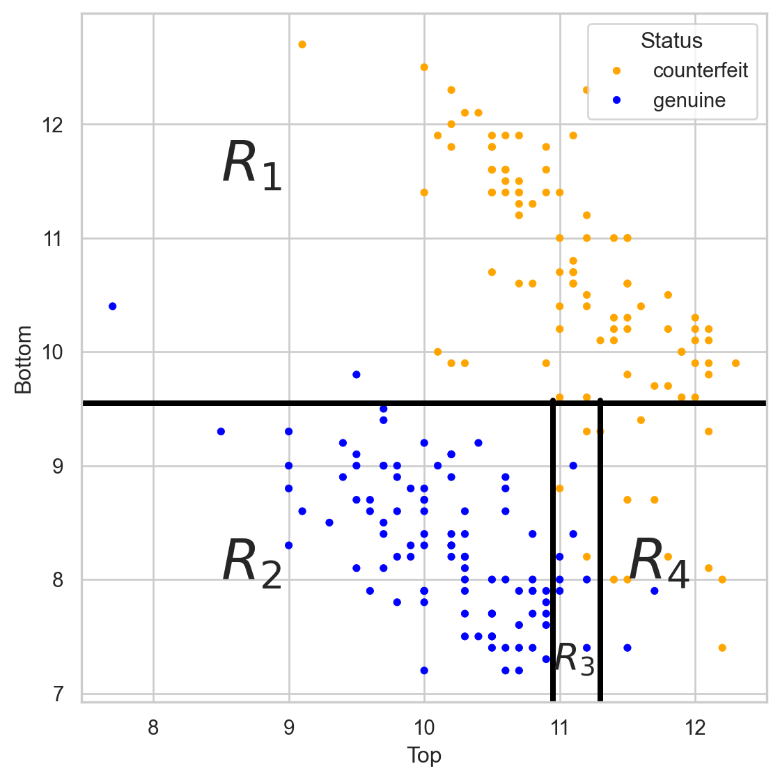
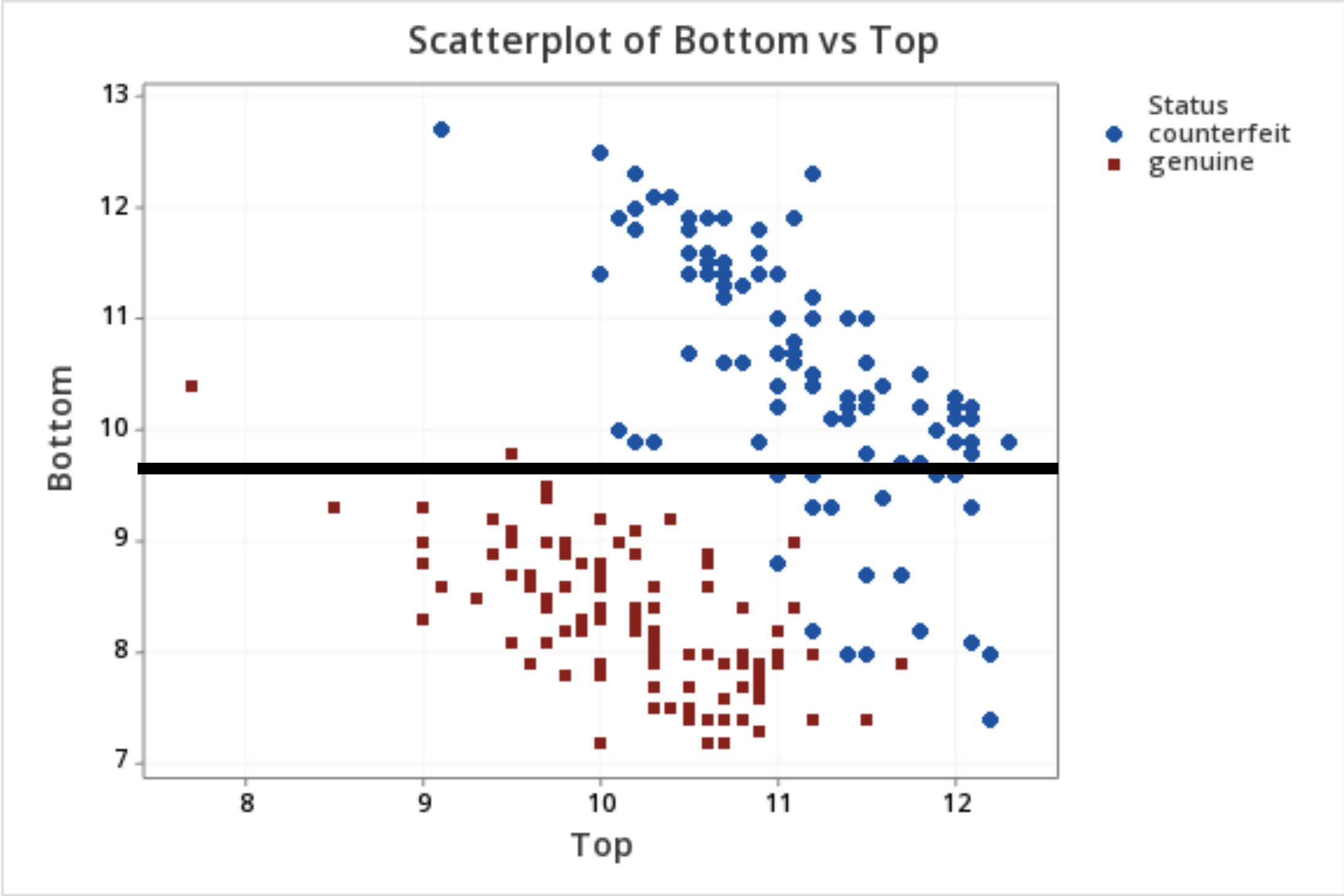
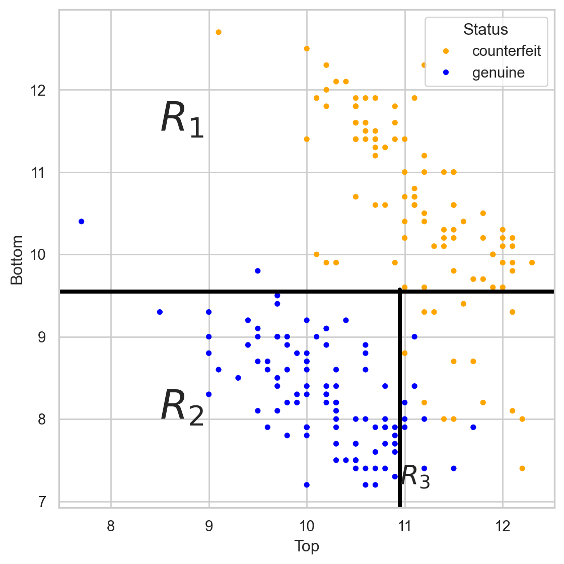
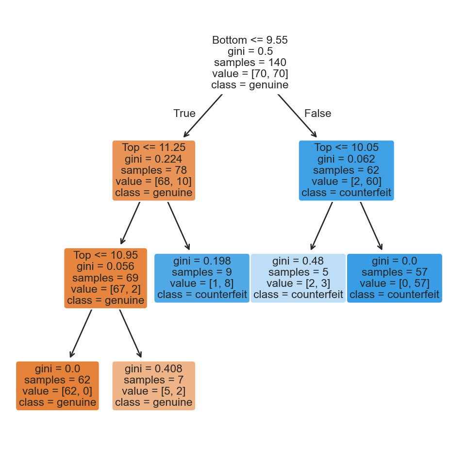
Example 1: Identifying Counterfeit Banknotes

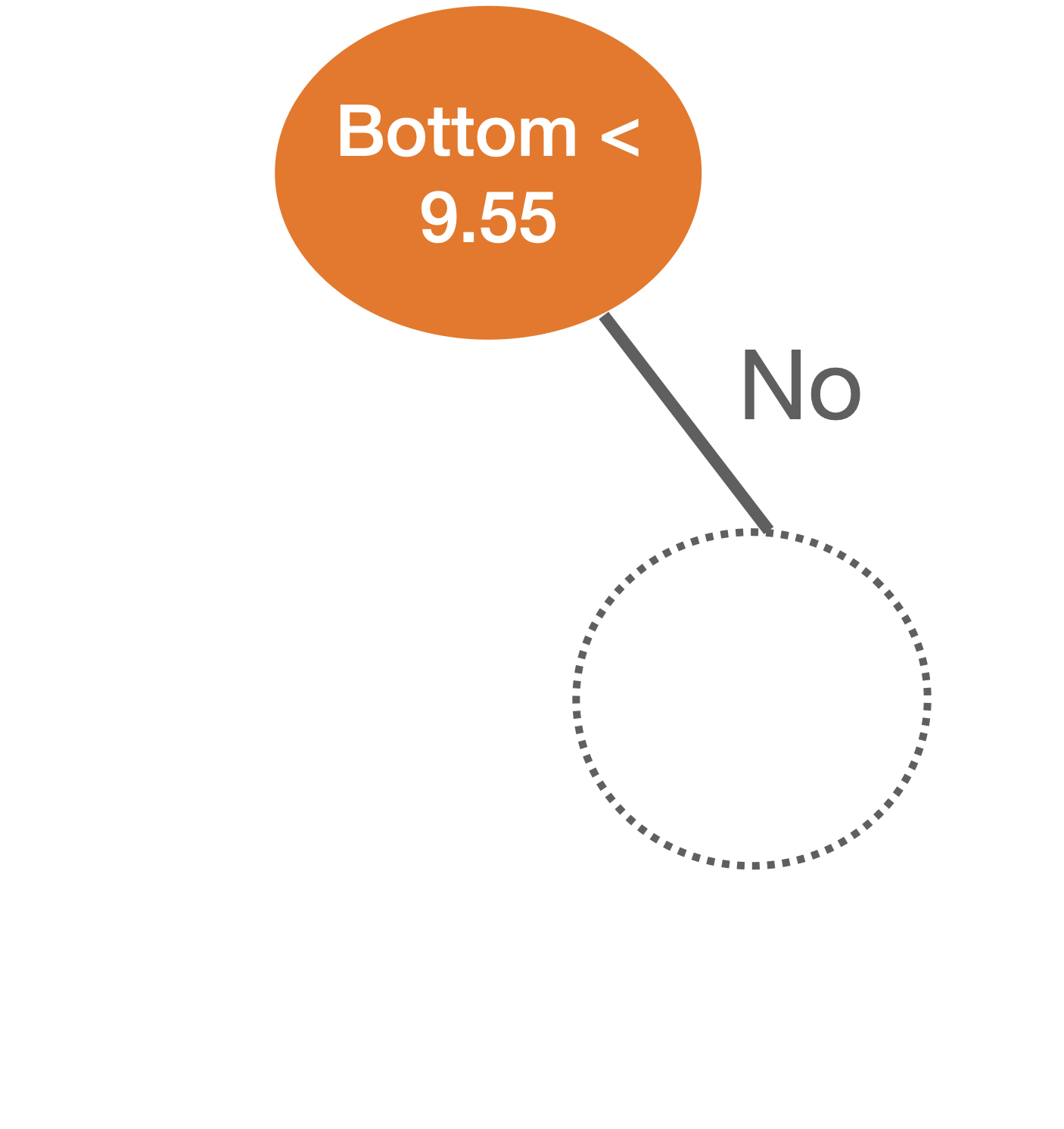
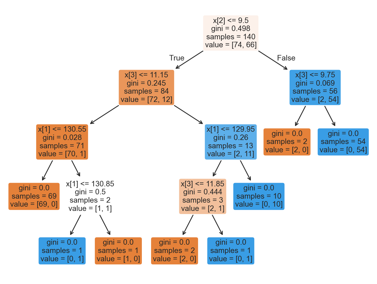
Basic idea of a decision tree
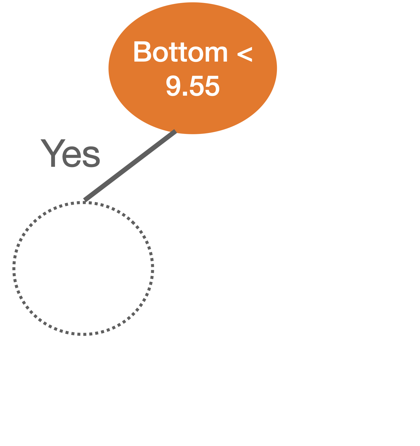
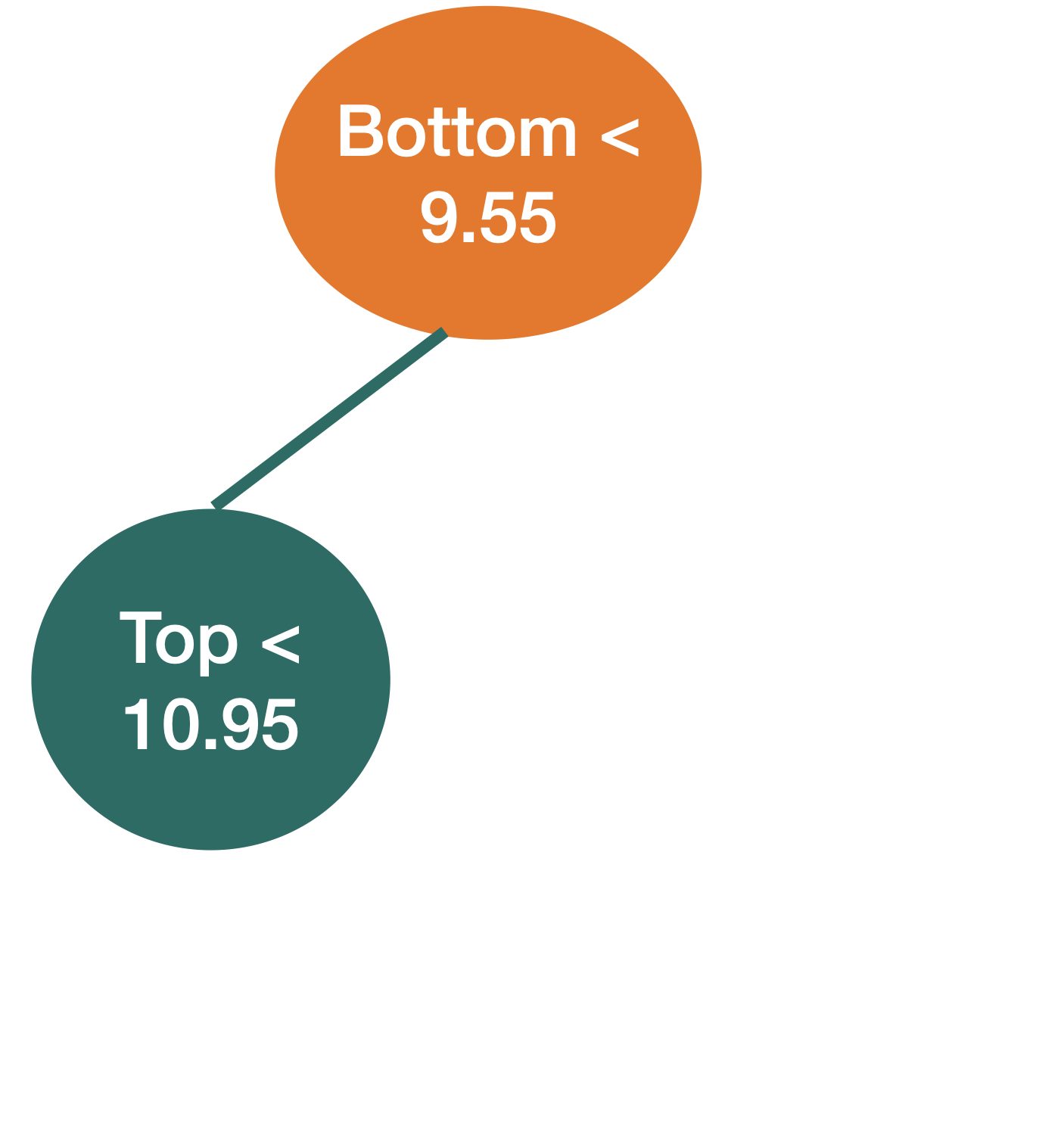
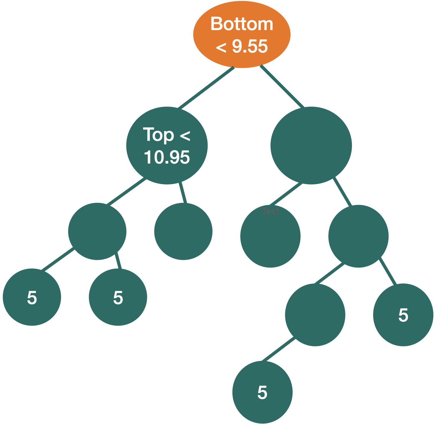
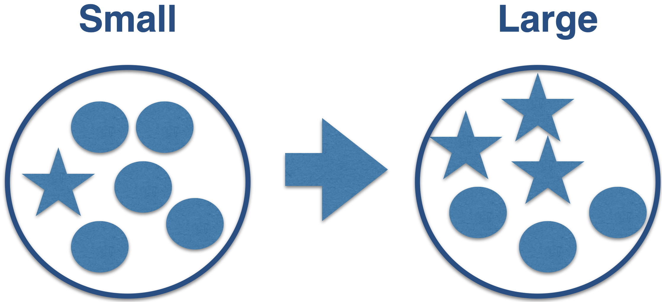
Stratify or segment the predictor space into several simpler regions.


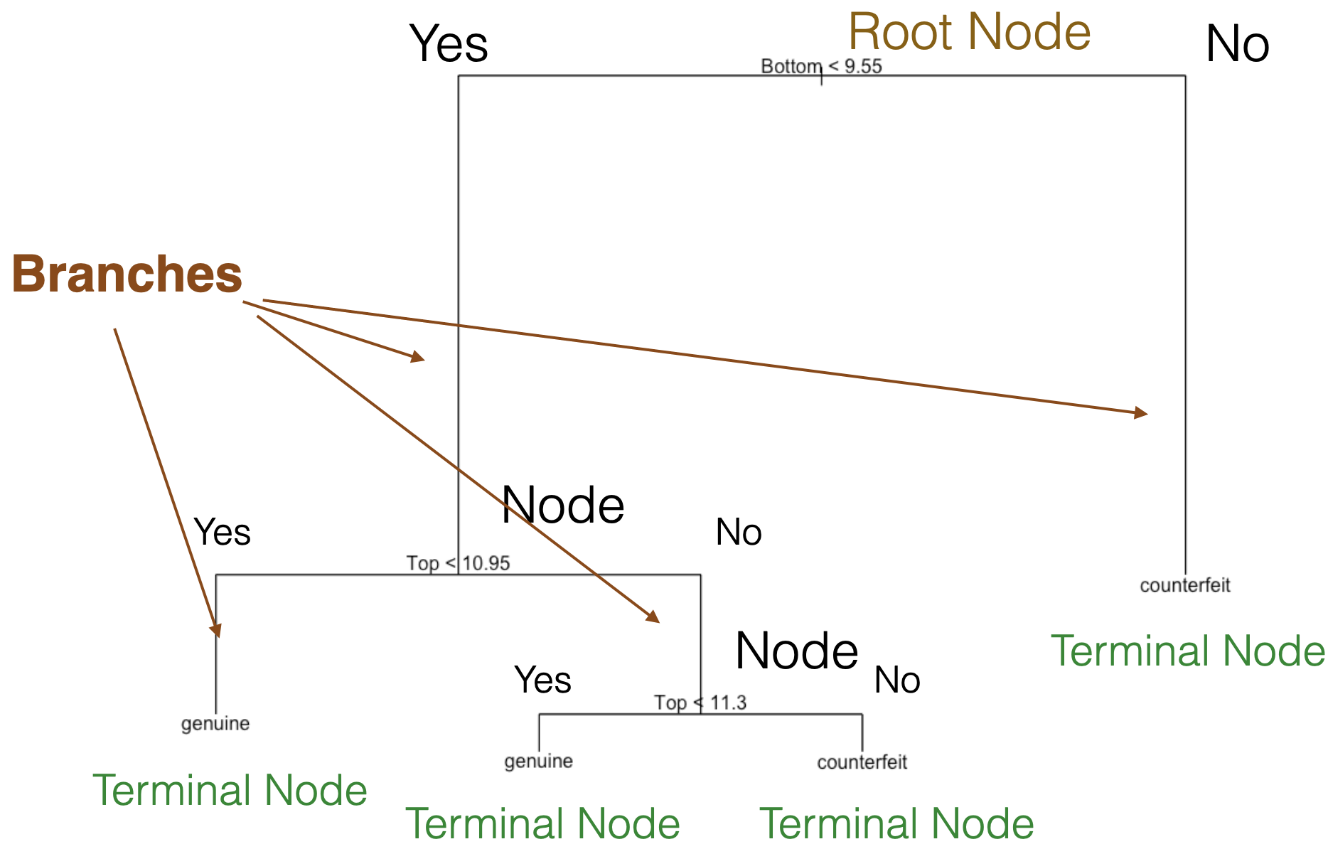


We repeat the partitioning process until:
- impurity does not improve in any of the terminal nodes, or
- each terminal node has no less than, say, 5 observations.
What is impurity?
Node impurity refers to the homogeneity of the response classes at that node.
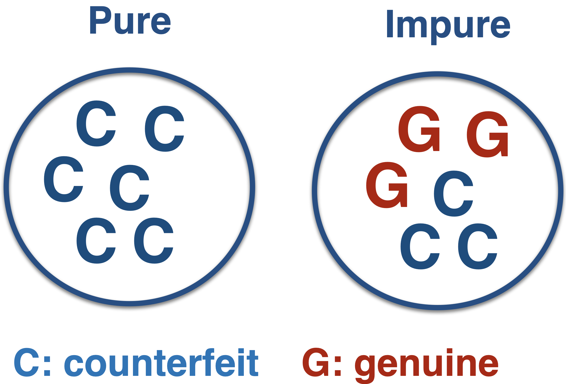
The CART algorithm minimizes impurity between tree nodes.
How do we measure impurity?
There are three different metrics for impurity:
Misclassification risk.
Cross entropy.
Gini impurity index.
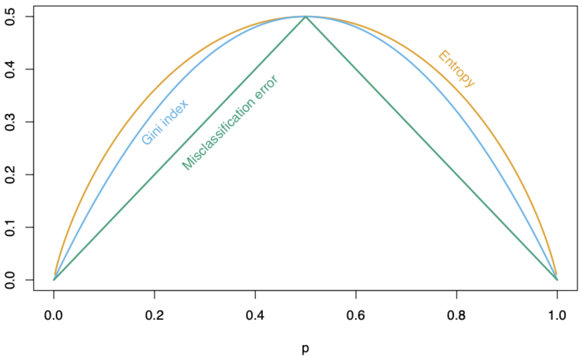
p: Proportion of elements in the target class
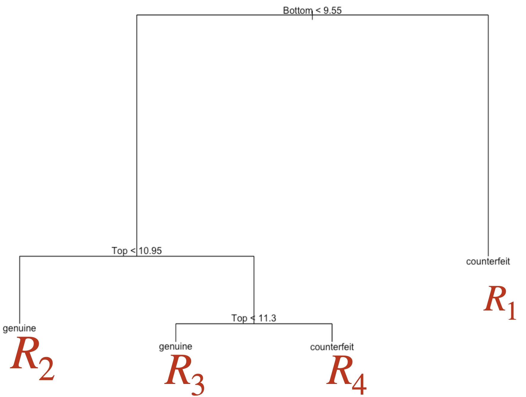
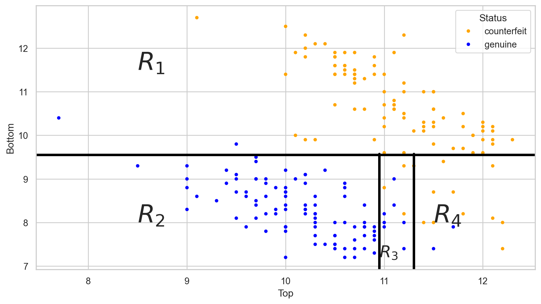
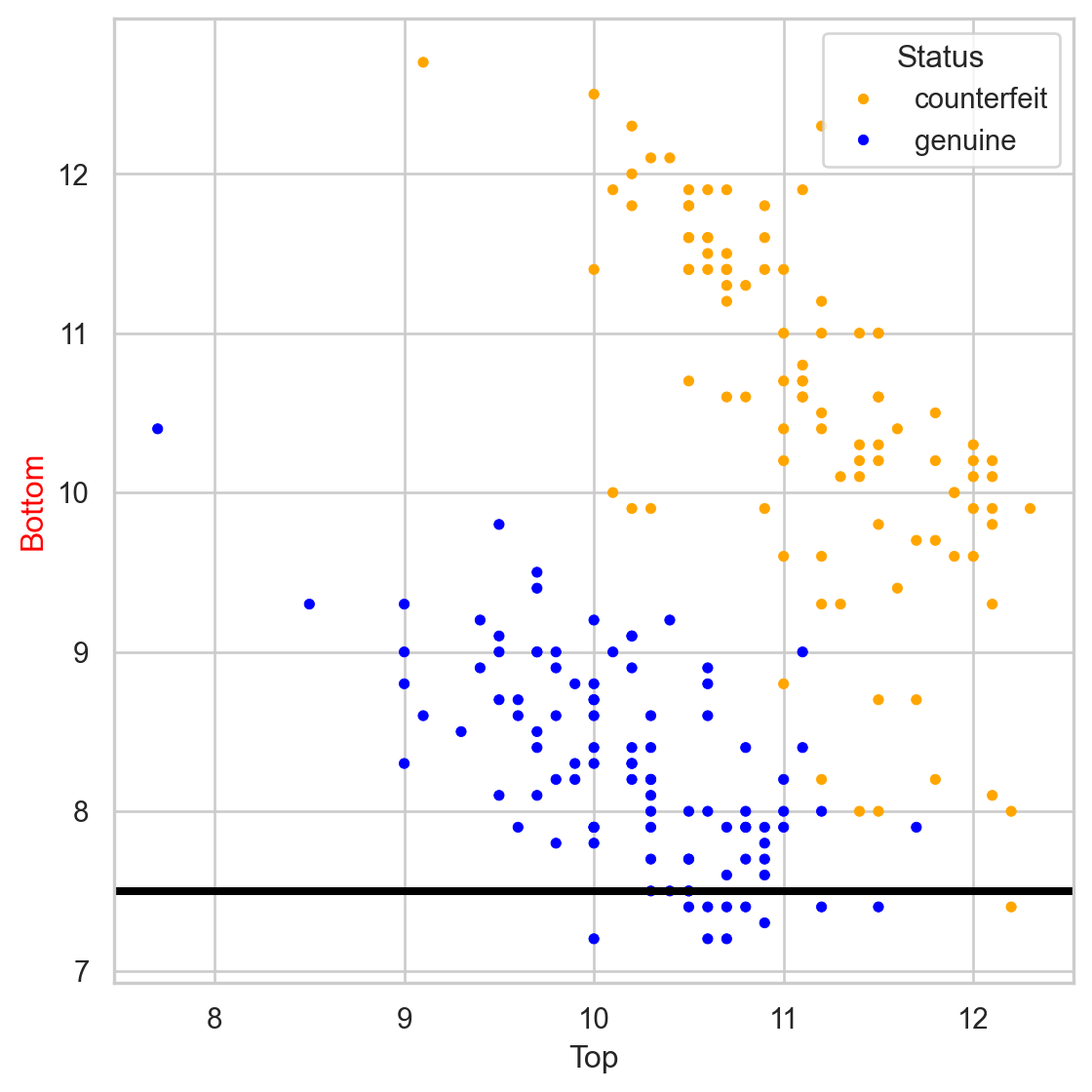
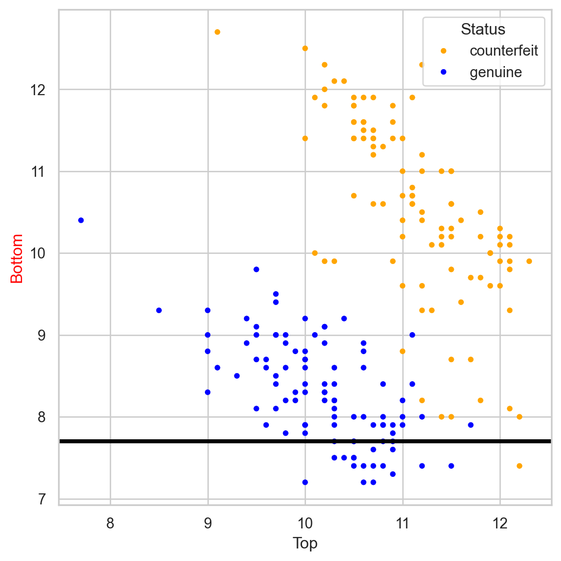
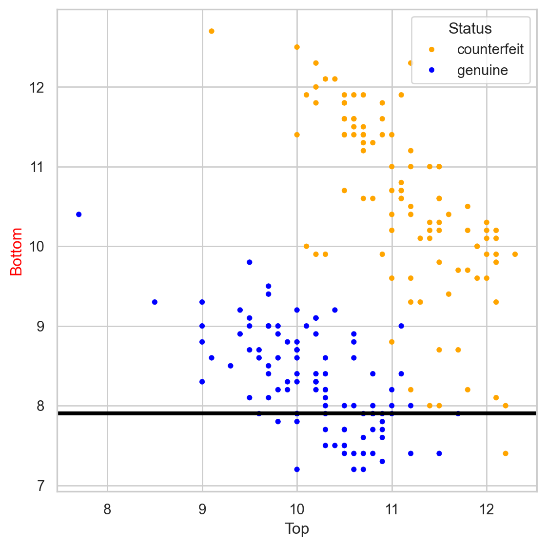
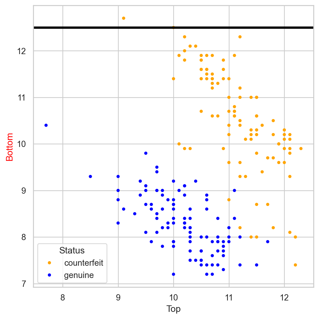
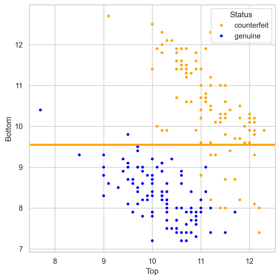
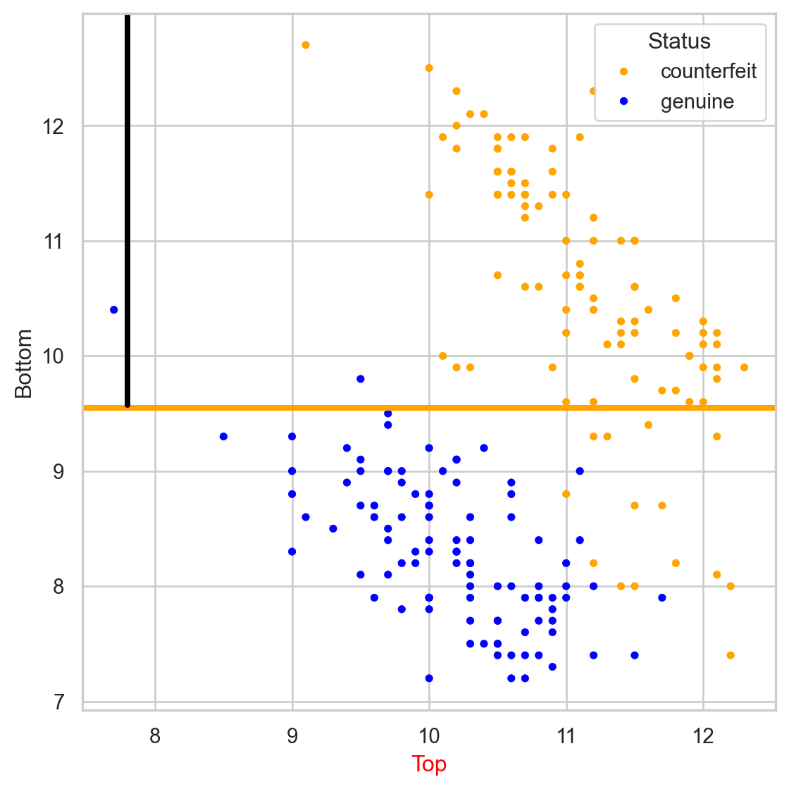
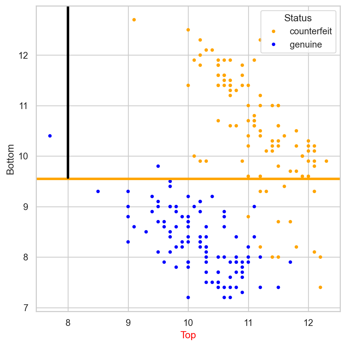
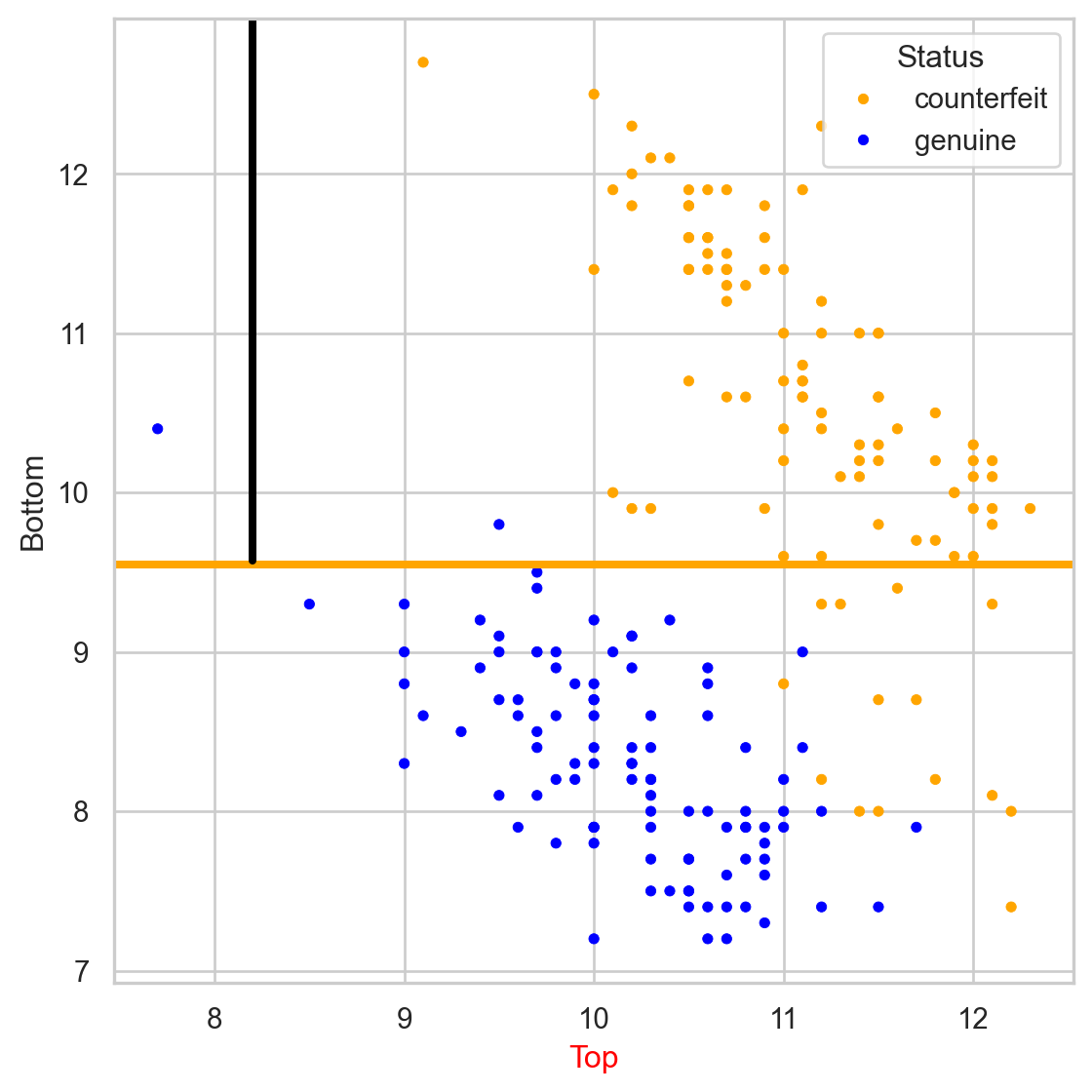
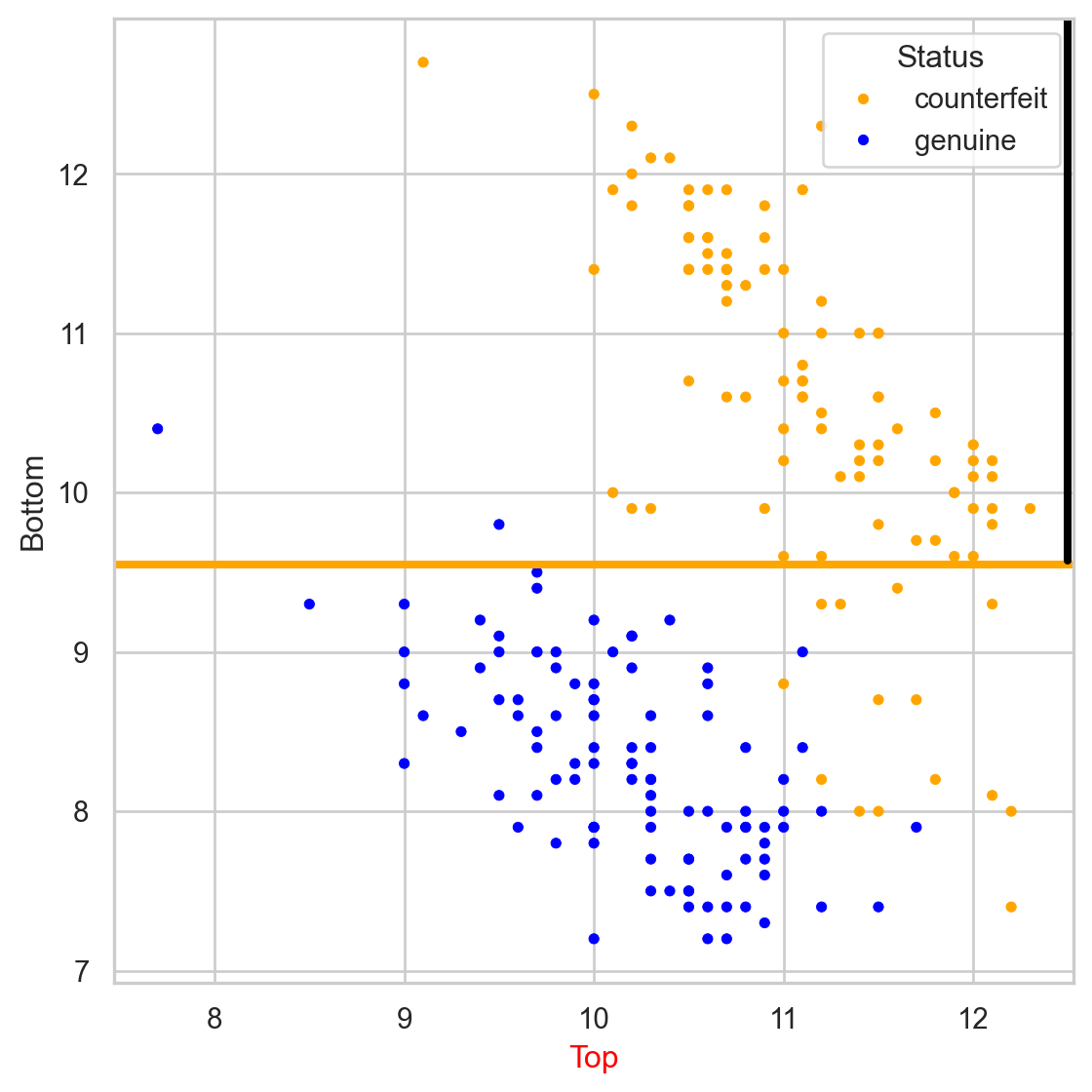
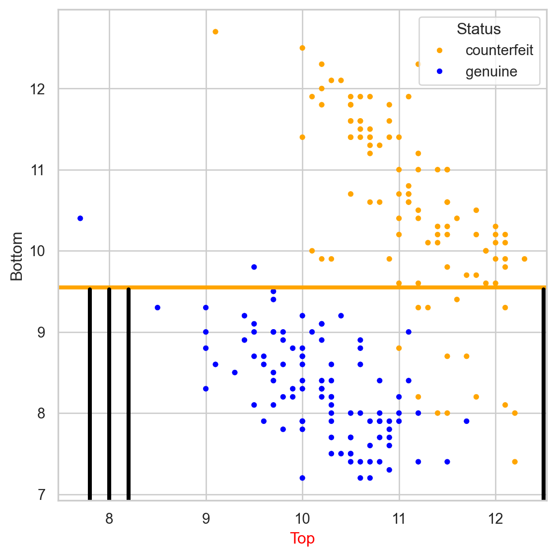
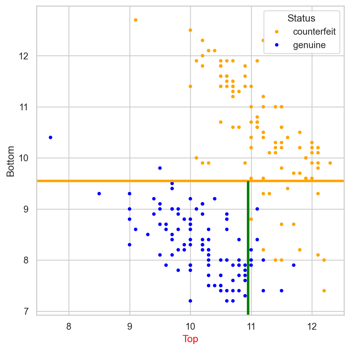
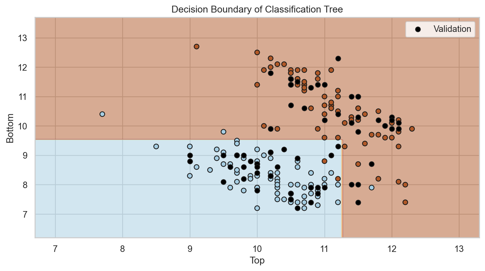
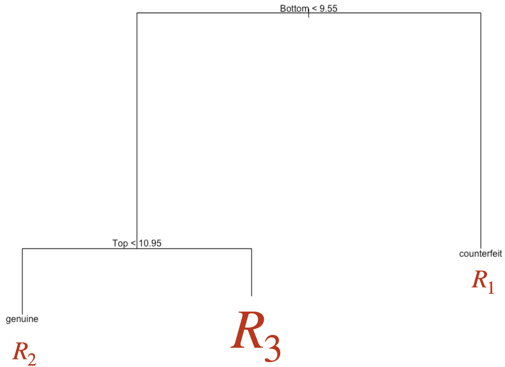
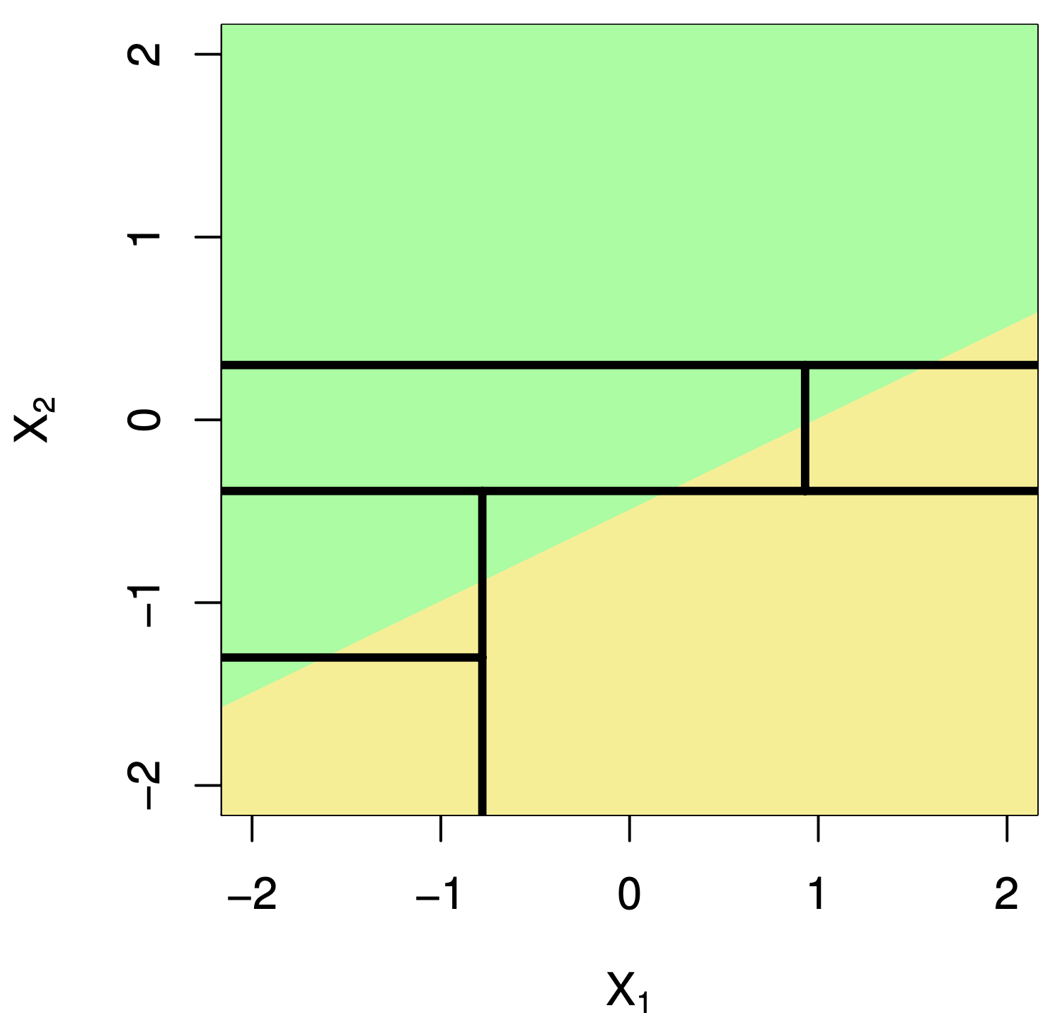
The tree in the predictor space
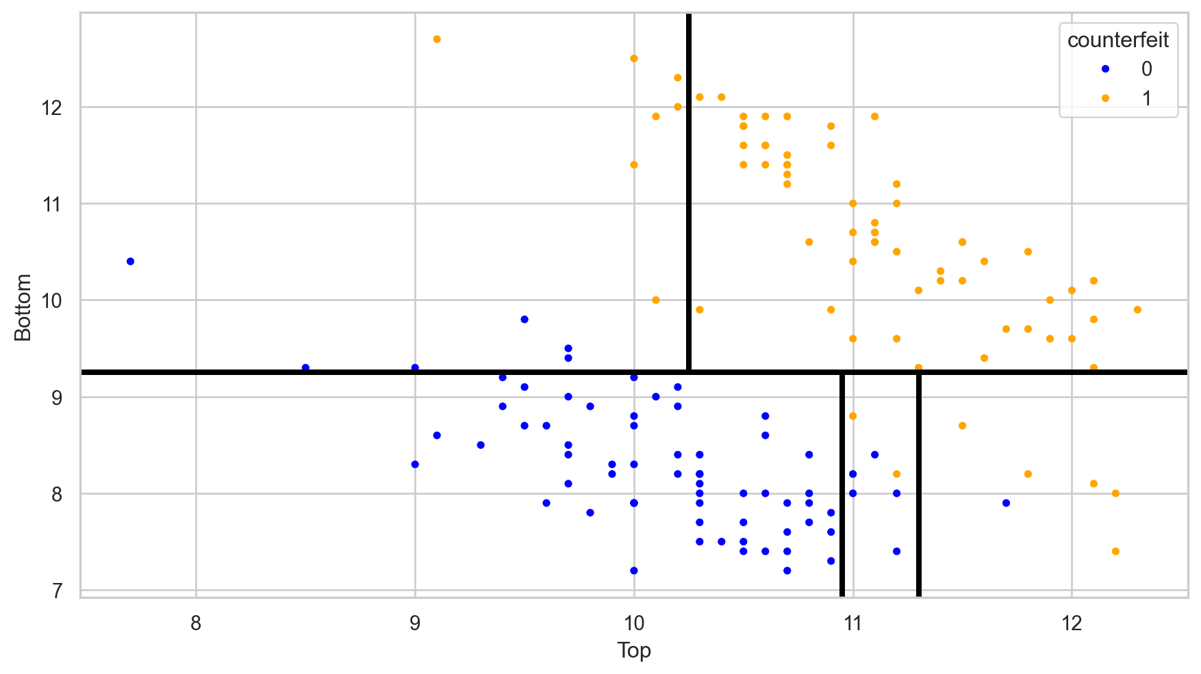
Visually
Let \((\hat{p}_0(\boldsymbol{x}), \hat{p}_1(\boldsymbol{x}))\) be the estimated probabilities.
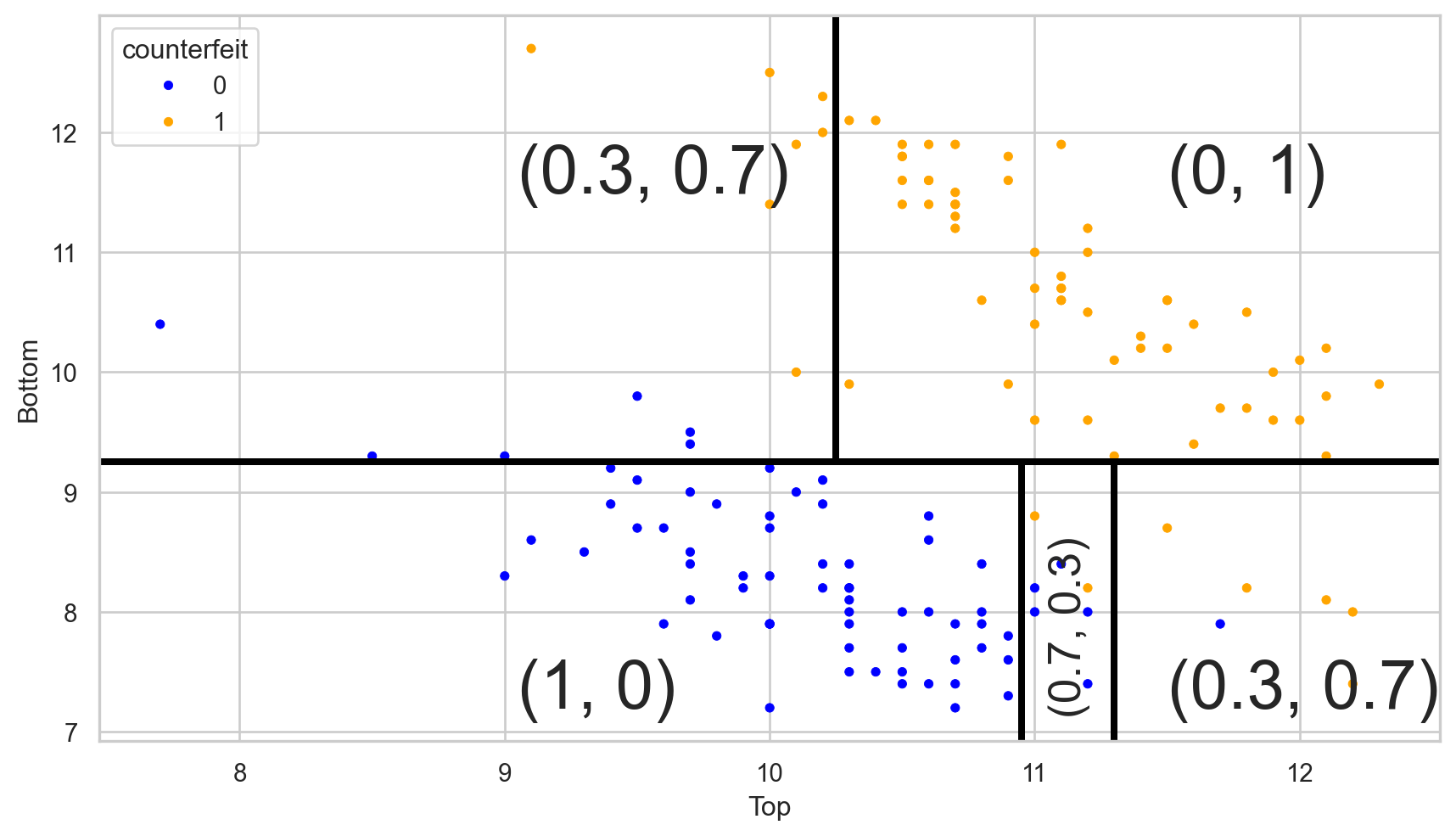
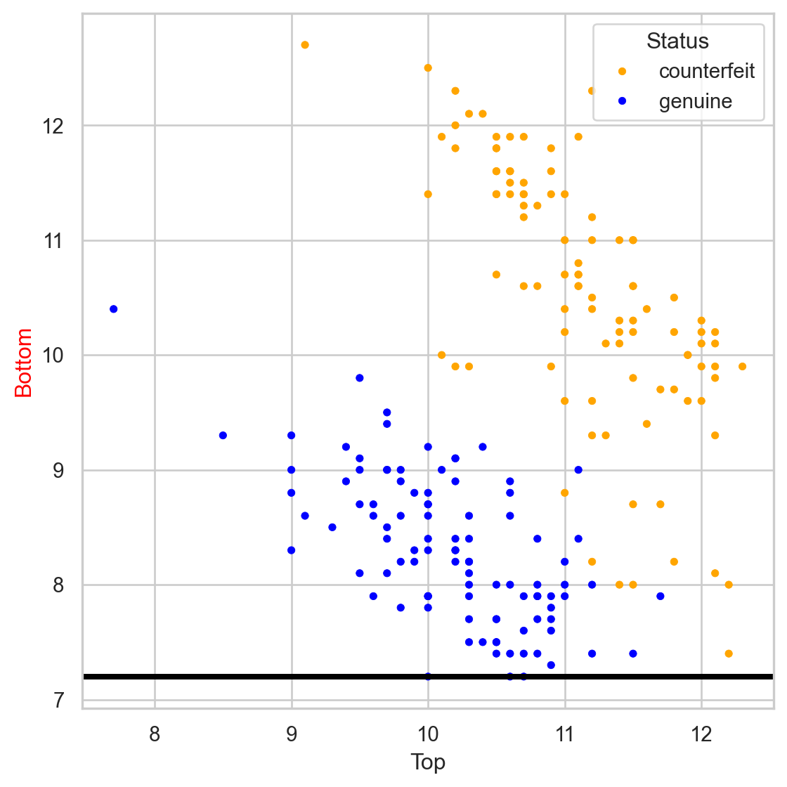
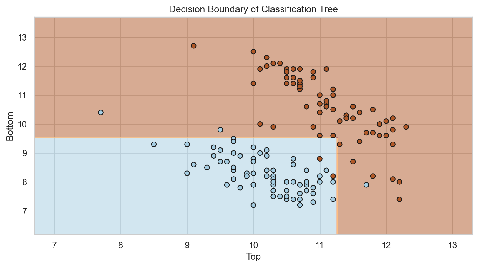
Simplified decision boundary
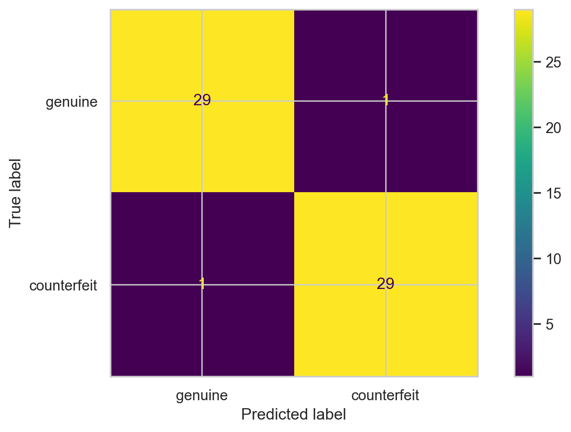
Confusion matrix
Table to evaluate the performance of a classifier.
Compares actual values with the predicted values of a classifier.
Useful for binary and multiclass classification problems.
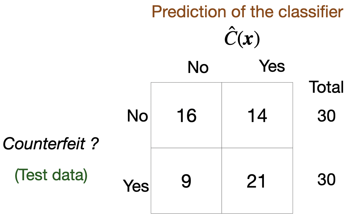
In Python
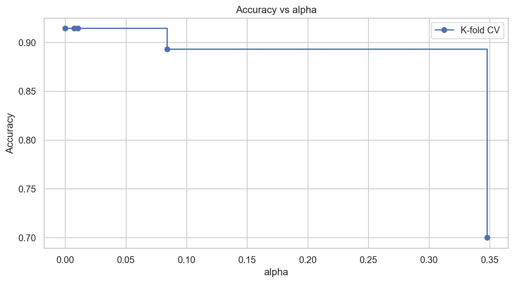
Pruning the tree
In some cases, we can optimize the performance of the tree by pruning it. That is, we collapse two internal (non-terminal) nodes.
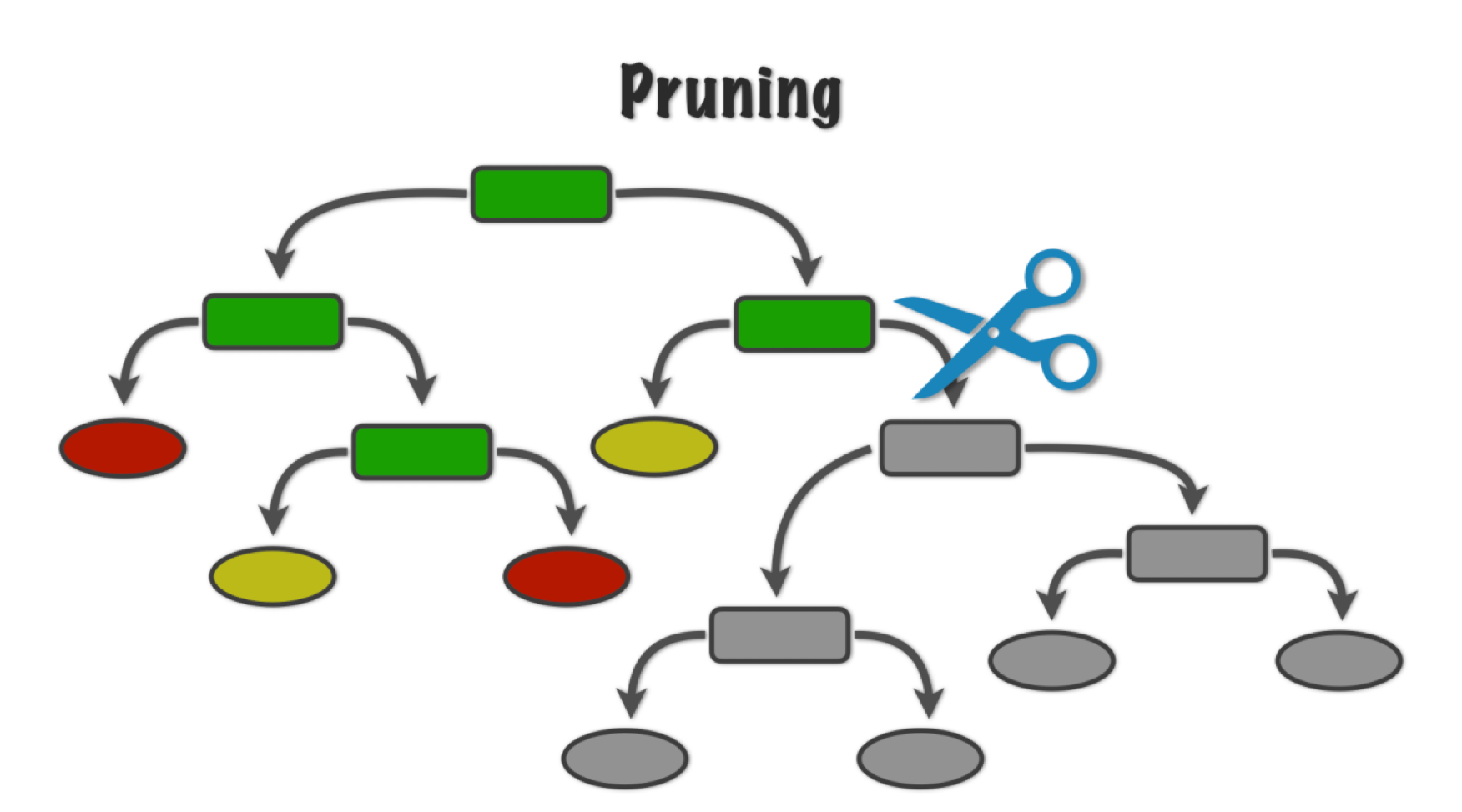
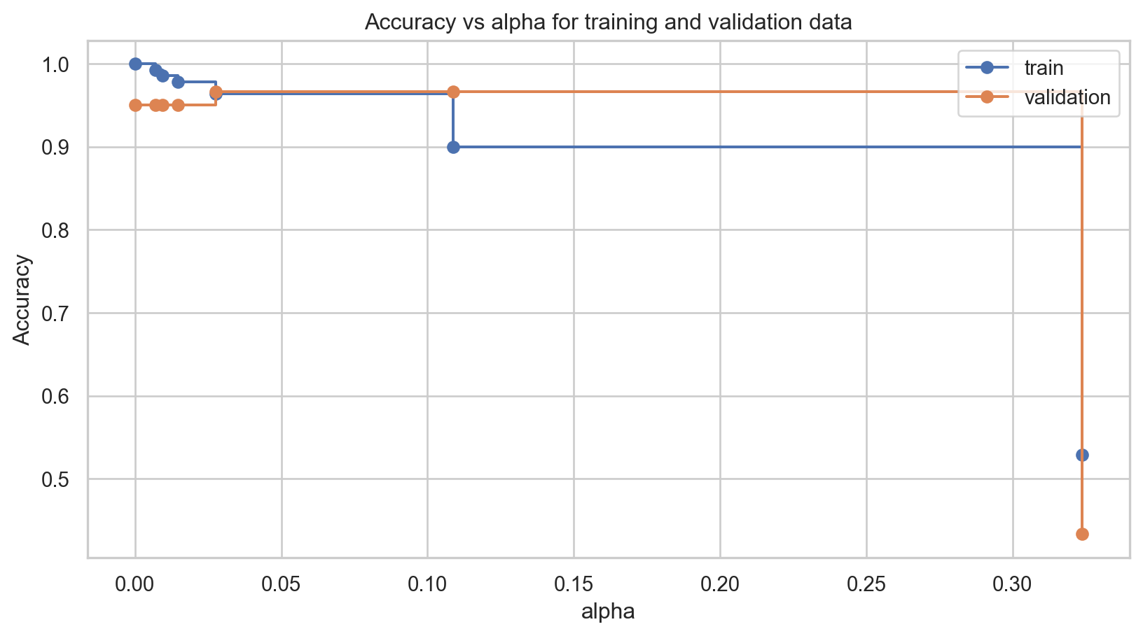
We visualize the results using the following plot.
Once this is done, we can visualize the small tree using the plot_tree() function.
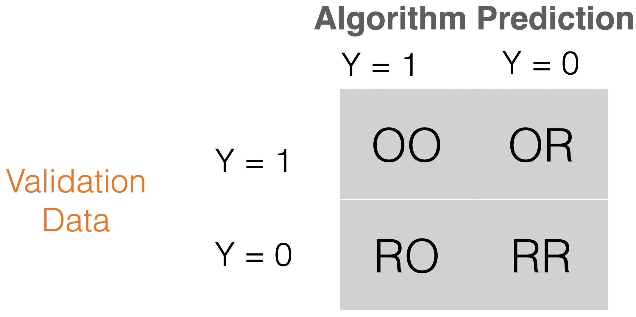
Sensitivity or recall = OO/(OO + OR) “How many records of the target class did we predict correctly?”
Precision = OO/(OO + RO) How many of the records we predicted as target class were classified correctly?
Type I error = RO/(RO + RR) “How many of the reference records did we incorrectly predict as targets?”
Disadvantages of decision trees
Decision trees have high variance. A small change in the training data can result in a very different tree.
It has trouble identifying simple data structures.
Comments on accuracy
Accuracy is easy to calculate and interpret.
It works well when the data set has a balanced class distribution (i.e., cases 1 and 0 are approximately equal).
However, there are situations in which identifying the target class is more important than the reference class.
For example, it is not ideal for unbalanced data sets. When one class is much more frequent than the other, accuracy can be misleading.