# Importing necessary libraries
import pandas as pd
import matplotlib.pyplot as plt
import seaborn as sns
from sklearn.model_selection import train_test_split, GridSearchCV
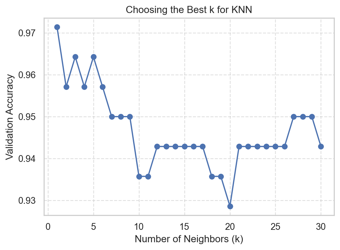
from sklearn.neighbors import KNeighborsClassifier
from sklearn.preprocessing import StandardScaler
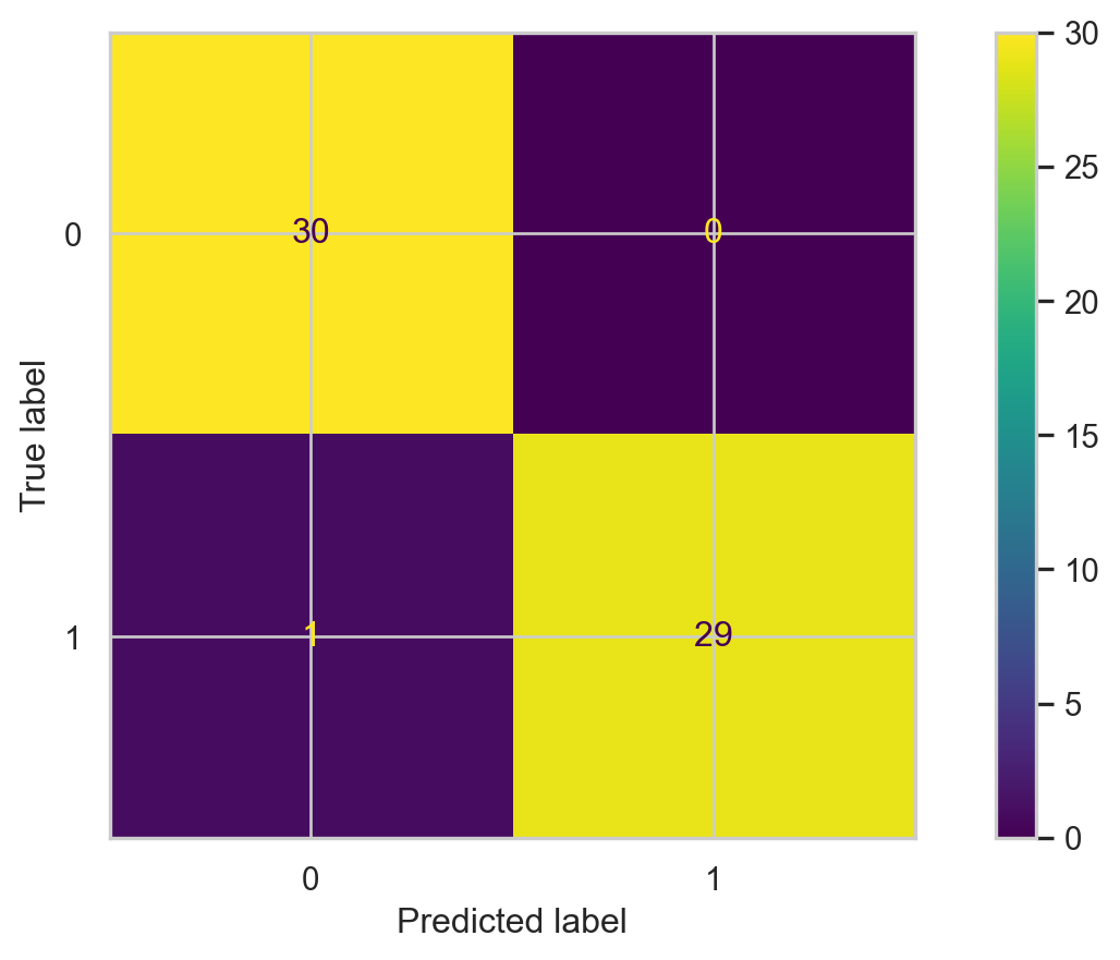
from sklearn.metrics import confusion_matrix, ConfusionMatrixDisplay
from sklearn.metrics import accuracy_scoreMain data science problems
Regression Problems. The response is numerical. For example, a person’s income, the value of a house, or a patient’s blood pressure.
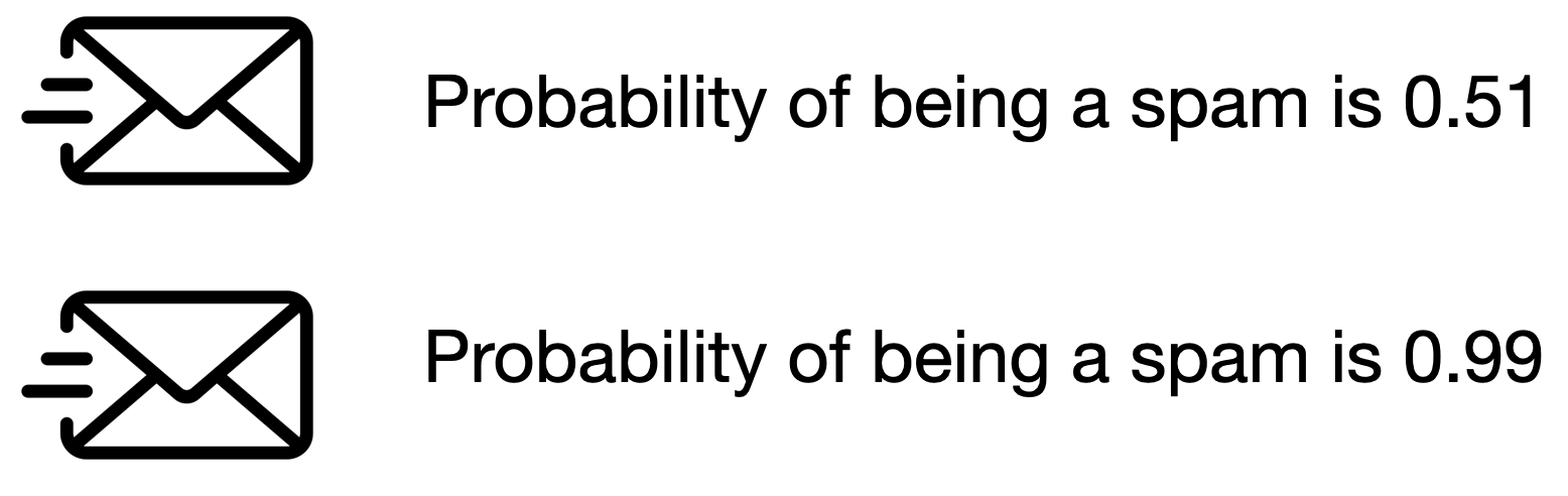
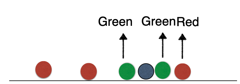
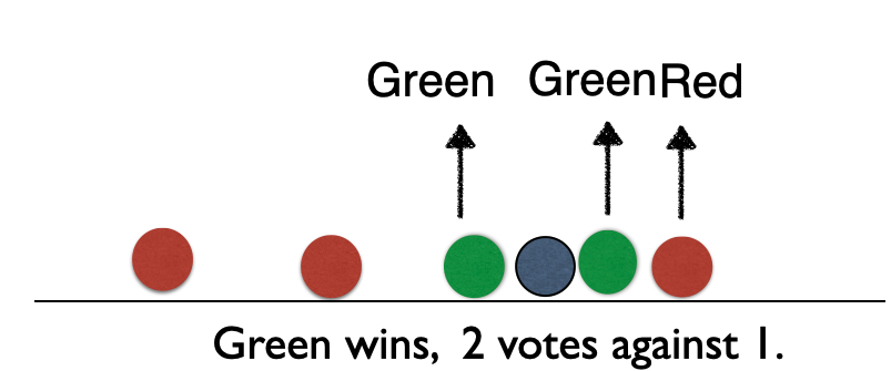
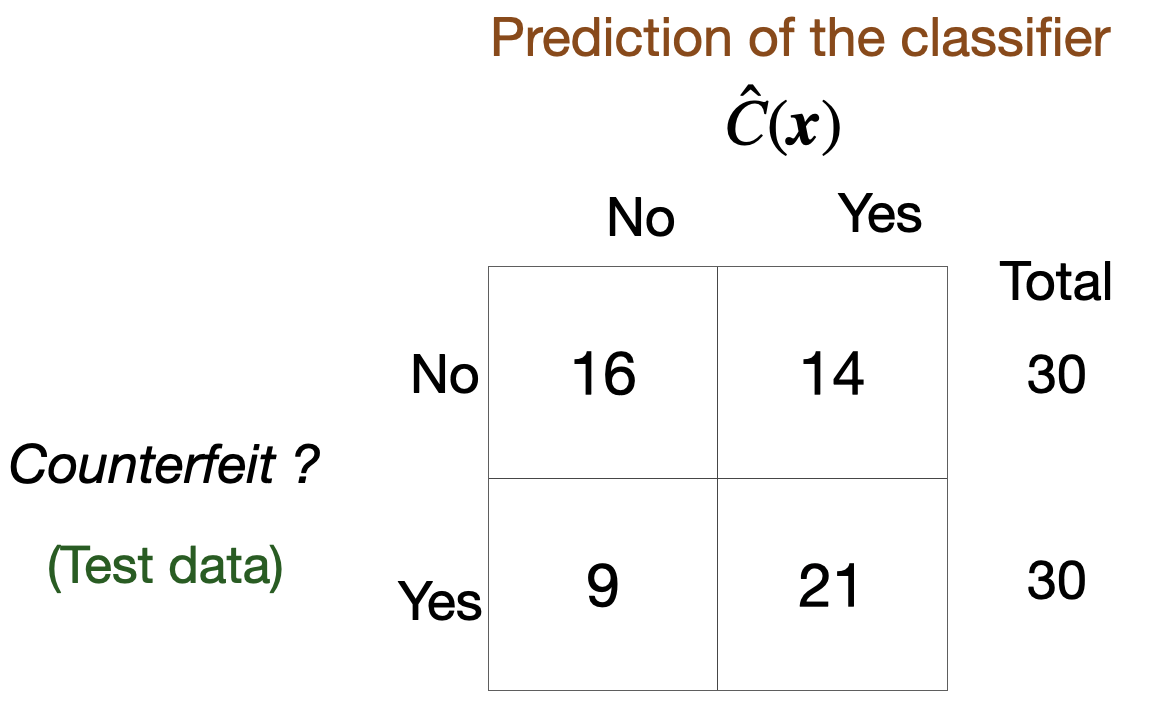
Classification Problems. The response is categorical and involves K different categories. For example, the brand of a product purchased (A, B, C) or whether a person defaults on a debt (yes or no).
The predictors (\(\boldsymbol{X}\)) can be numerical or categorical.