Additional Topics

IN5148: Statistics and Data Science with Applications in Engineering

Alan R. Vazquez

Department of Industrial Engineering

Agenda

Linear Models with Categorical Predictors
Another Example

Load the libraries

Let’s import scikit-learn into Python together with the other relevant libraries.

import pandas as pd
import seaborn as sns
import matplotlib.pyplot as plt
import statsmodels.api as sm
from sklearn.linear_model import LinearRegression
from sklearn.preprocessing import StandardScaler
from sklearn.model_selection import train_test_split
from sklearn.metrics import root_mean_squared_error

We will not use all the functions from the scikit-learn library. Instead, we will use specific functions from the sub-libraries preprocessing, model_selection, and metrics.

Linear Models with Categorical Predictors

Categorical predictors

A categorical predictor takes on values that are categories, say, names or labels.
Their use in regression requires dummy variables, which are quantitative variables.
When a categorical predictor has more than two levels, a single dummy variable cannot represent all possible categories.
In general, a categorical predictor with $k$ categories requires $k-1$ dummy variables.

Dummy coding

Traditionally, dummy variables are binary variables which can only take the values 0 and 1.
This approach implies a reference category. Specifically, the category that results when all dummy variables equal 0.
This coding impacts the interpretation of the model coefficients:
- $\beta_0$ is the mean response under the reference category.
- $\beta_j$ is the amount of increase in the mean response when we change from the reference category to another category.

Example 1

The auto data set includes a categorical variable “Origin” which shows the origin of each car.

# Load the Excel file into a pandas DataFrame.
auto_data = pd.read_excel("auto.xlsx")

# Set categorical variables.
auto_data['origin'] = pd.Categorical(auto_data['origin'])

In this section, we will consider the auto_data as our training dataset.

Dataset

(auto_data
.filter(['mpg', 'origin'])
).head(6)

	mpg	origin
0	18.0	American
1	15.0	American
2	18.0	American
3	16.0	American
4	17.0	American
5	15.0	American

Dummy variables

Origin has 3 categories: European, American, Japanese.

So, 2 dummy variables are required:

\[d_1 = \begin{cases} 1 \text{ if car is European}\\ 0 \text{ if car is not European} \end{cases} \text{ and }\]

\[d_2 = \begin{cases} 1 \text{ if car is Japanese}\\ 0 \text{ if car is not Japanese} \end{cases}.\]

“American” acts as the reference category.

The dataset with the dummy variables looks like this:

origin	$d_1$	$d_2$
American	0	0
American	0	0
European	1	0
European	1	0
American	0	0
Japanese	0	1
$\vdots$	$\vdots$	$\vdots$

Linear regression model

\[\hat{Y}_i= \hat{\beta}_0 + \hat{\beta}_1 d_{1i} + \hat{\beta}_2 d_{2i} \ \text{for} \ i=1,\ldots,n.\]

$\hat{Y}_i$ is the i-th predicted response.
$d_{1i}$ is 1 if the i-th observation is from a European car, and 0 otherwise.
$d_{2i}$ is 1 if the i-th observation is from a Japanese car, and 0 otherwise.

Model coefficients

\[ \hat{Y}_i= \hat{\beta}_0 + \hat{\beta}_1 d_{1i} + \hat{\beta}_2 d_{2i} \]

$\hat{\beta}_0$ is the mean response (mpg) for American cars.
$\hat{\beta}_1$ is the amount of increase in the mean response when changing from an American to a European car.
$\hat{\beta}_2$ is the amount of increase in the mean response when changing from an American to a Japanese car.

Alternatively, we can write the regression model as:

\[ \hat{Y}_i= \hat{\beta}_0+\hat{\beta}_1 d_{1i} +\hat{\beta}_2 d_{2i} = \begin{cases} \hat{\beta}_0+\hat{\beta}_1 +\hat{\beta}_i \text{ if car is European}\\ \hat{\beta}_0+\hat{\beta}_2 \text{ if car is Japanese} \\ \hat{\beta}_0 \;\;\;\;\;\;\ \text{ if car is American} \end{cases} \]

Given this model representation:

$\hat{\beta}_0$ is the mean mpg for American cars,
$\hat{\beta}_1$ is the difference in the mean mpg between European and American cars, and
$\hat{\beta}_2$ is the difference in the mean mpg between Japanese and American cars.

In Python

We follow three steps to fit a linear model with a categorical predictor. First, we compute the dummy variables.

# Create linear regression object
dummy_X_train = pd.get_dummies(auto_data['origin'], drop_first = True, 
                            dtype = 'int')

Next, we construct the response column.

# Create response vector
Y_train = auto_data['mpg']

Finally, we fit the model using scikit-learn.

# 1. Create the linear regression model
LRmodel = LinearRegression()

# 2. Fit the model.
LRmodel.fit(dummy_X_train, Y_train)

# 3. Show estimated coefficients.
print("Intercept:", LRmodel.intercept_)
print("Coefficients:", LRmodel.coef_)

Intercept: 20.033469387755094
Coefficients: [ 7.56947179 10.41716352]

Analysis of covariance

Models that mix categorical and numerical predictors are sometimes referred to as analysis of covariance (ANCOVA) models.

Example (cont): Consider the predictor weight ($X$).

\[\hat{Y}_i= \hat{\beta}_0 + \hat{\beta}_1 d_{1i} + \hat{\beta}_2 d_{2i} + \hat{\beta}_3 X_{i},\]

where $X_i$ denotes the i-th observed value of weight and $\hat{\beta}_3$ is the coefficient of this predictor.

ANCOVA model

The components of the ANCOVA model are individual functions of the coefficients.

To gain insight into the model, we write it as follows:

\[ \begin{align} \hat{Y}_i &= \hat{\beta}_0+\hat{\beta}_1 d_{1i} +\hat{\beta}_2 d_{2i} + \hat{\beta}_3 X_{i} \\ &= \begin{cases} (\hat{\beta}_0+\hat{\beta}_1) + \hat{\beta}_3 X_{i} & \text{ if car is European} \\ (\hat{\beta}_0+\hat{\beta}_2) + \hat{\beta}_3 X_{i} & \text{ if car is Japanese} \\ \hat{\beta}_0 + \hat{\beta}_3 X_{i} \;\;\;\;\;\;\;\;\ & \text{ if car is American} \\ \end{cases}. \end{align} \]

The models have different intercepts but the same slope.

To estimate $\hat{\beta}_0$, $\hat{\beta}_1$, $\hat{\beta}_2$ and $\hat{\beta}_3$, we use least squares.
We could make individual inferences on $\beta_1$ and $\beta_2$ using t-tests in the statsmodels library.
However, better tests are possible such as overall and partial F-tests (not discussed here).

In Python

To fit an ANCOVA model, we use similar steps as before. The only extra step is to concatenate the data with the dummy variables and the numerical predictor using the function concat() from pandas.

# Concatenate the two data sets.
X_train = pd.concat([dummy_X_train, auto_data['weight']], axis = 1)

# 1. Create the linear regression model
LRmodel_ancova = LinearRegression()

# 2. Fit the model.
LRmodel_ancova.fit(X_train, Y_train)

The estimated model is shown below.

# 3. Show estimated coefficients.
print("Intercept:", LRmodel_ancova.intercept_)
print("Coefficients:", LRmodel_ancova.coef_)

Intercept: 43.732236151632975
Coefficients: [ 0.97090559  2.3271499  -0.00702708]

Another Example

Example 2

The “BostonHousing.xlsx” contains data collected by the US Bureau of the Census concerning housing in the area of Boston, Massachusetts. The dataset includes data on 506 census housing tracts in the Boston area in 1970s.

The goal is to predict the median house price in new tracts based on information such as crime rate, pollution, and number of rooms.

The response is the median value of owner-occupied homes in $1000s, contained in the column MEDV.

The predictors

CRIM: per capita crime rate by town.
ZN: proportion of residential land zoned for lots over 25,000 sq.ft.
INDUS: proportion of non-retail business acres per town.
CHAS: Charles River dummy variable (= 1 if tract bounds river; 0 otherwise).
NOX: nitrogen oxides concentration (parts per 10 million).
RM: average number of rooms per dwelling.
AGE: proportion of owner-occupied units built prior to 1940.
DIS: weighted mean of distances to five Boston employment centers
RAD: index of accessibility to radial highways.
TAX: full-value property-tax rate per $10,000.
PTRATIO: pupil-teacher ratio by town.
LSTAT: lower status of the population (percent).

Read the dataset

We read the dataset and set the variable CHAS as categorical.

# Load Excel file (make sure the file is in your Colab)
Boston_data = pd.read_excel('BostonHousing.xlsx')

# Drop the categorical variable.
Boston_data['CHAS'] = pd.Categorical(Boston_data['CHAS'])
Boston_data['RAD'] = pd.Categorical(Boston_data['RAD'])

# Preview the dataset.
Boston_data.head(3)

	CRIM	ZN	INDUS	CHAS	NOX	RM	AGE	DIS	RAD	TAX	PTRATIO	LSTAT	MEDV
0	0.00632	18.0	2.31	No	0.538	6.575	65.2	4.0900	Low	296	15.3	4.98	24.0
1	0.02731	0.0	7.07	No	0.469	6.421	78.9	4.9671	Low	242	17.8	9.14	21.6
2	0.02729	0.0	7.07	No	0.469	7.185	61.1	4.9671	Low	242	17.8	4.03	34.7

Train and validation data

We split the dataset into a training and a validation dataset using the function train_test_split() from scikit-learn.

# Set full matrix of predictors.
X_full = Boston_data.drop(columns = ['MEDV']) 

# Set full matrix of responses.
Y_full = Boston_data['MEDV']

# Split the dataset into training and validation.
X_train, X_valid, Y_train, Y_valid = train_test_split(X_full, Y_full, 
                                                      test_size=0.3,
                                                      random_state = 59227)

The parameter test_size sets the portion of the dataset that will go to the validation set. It is usually 0.3 or 0.2.

Transform the categorical predictors

Before we continue, let’s turn the categorical predictors into dummy variables

# Transform categorical predictors into dummy variables
Boston_X_train = pd.get_dummies(X_train, drop_first = True, dtype = 'int')
Boston_X_train.head(3)

	CRIM	ZN	INDUS	NOX	RM	AGE	DIS	TAX	PTRATIO	LSTAT	RAD_Medium
452	5.09017	0.0	18.10	0.713	6.297	91.8	2.3682	666	20.2	17.27	0
317	0.24522	0.0	9.90	0.544	5.782	71.7	4.0317	304	18.4	15.94	1
352	0.07244	60.0	1.69	0.411	5.884	18.5	10.7103	411	18.3	7.79	1

Fit a model using training data

We train a linear regression model to predict the MEDV in terms of the 12 predictors using functions from scikit-learn.

# 1. Create the linear regression model
LRmodel = LinearRegression()

# 2. Fit the model.
LRmodel.fit(Boston_X_train, Y_train)

# 3. Show estimated coefficients.
print("Intercept:", LRmodel.intercept_)
print("Coefficients:", LRmodel.coef_)

Intercept: 37.516763561108434
Coefficients: [-5.31702151e-02  4.42408175e-02  8.46402739e-02 -1.19782458e+01
  3.82114415e+00  1.77709868e-02 -1.25752076e+00 -7.33041781e-03
 -9.14794029e-01 -7.17544266e-01  5.25221827e+00 -2.04793579e+00
 -2.47739812e+00]

Brief Residual Analysis

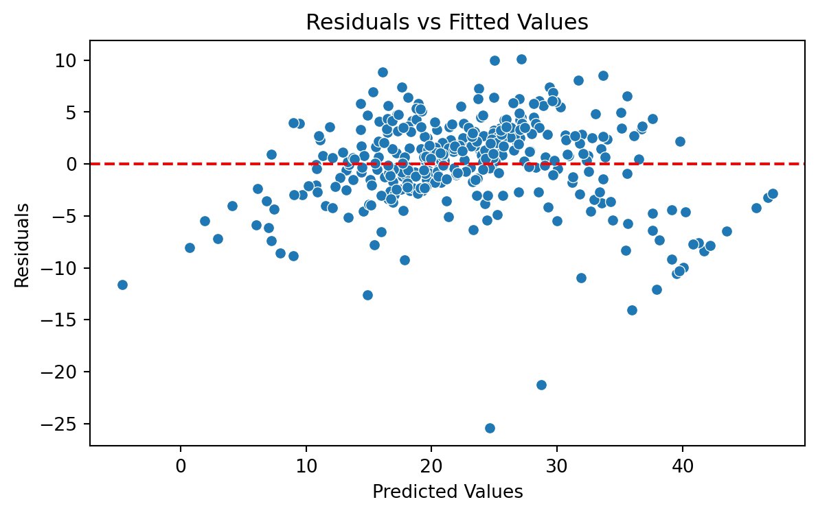
We evaluate the model using a “Residual versus Fitted Values” plot. The plot does not show concerning patterns in the residuals. So, we assume that the model satisfies the assumption of constant variance.

Validation Mean Squared Error

When the response is numeric, the most common evaluation metric is the validation Root Mean Squared Error (RMSE):

\[ \left(\frac{1}{n_{v}} \sum_{i=1}^{n_{v}} \left( Y_i - \hat{Y}_i \right)^2 \right)^{1/2} \]

where $(Y_1, \boldsymbol{X}_1), \ldots, (Y_{n_{v} }, \boldsymbol{X}_{n_{v}} )$ are the $n_{v}$ observations in the validation dataset, and $\hat{Y}_i = \hat{\beta}_0 + \hat{\beta}_1 X_{i1} + \hat{\beta}_2 X_{i2} + \cdots + \hat{\beta}_p X_{ip}$ is the model prediction of the i-th response.

Recall that …

The RMSE is in the same units as the response.
The RMSE value is interpreted as either how far (on average) the residuals are from zero.
It can also be interpreted as the average distance between the observed response values and the model predictions.

In Python

We first compute the predictions of our model on the validation dataset. To this end, we create the dummy variables of the categorical variables using the validation dataset.

Boston_X_val = pd.get_dummies(X_valid, drop_first = True, dtype = 'int')
Boston_X_val.head(3)

	CRIM	INDUS	NOX	RM	AGE	DIS	TAX	PTRATIO	LSTAT
482	5.73116	18.1	0.532	7.061	77.0	3.4106	666	20.2	7.01
367	13.52220	18.1	0.631	3.863	100.0	1.5106	666	20.2	13.33
454	9.51363	18.1	0.713	6.728	94.1	2.4961	666	20.2	18.71

Now, we use the values of the predictors in this dataset and use it as input to our model. Our model then computes the prediction of the response for each combination of values of the predictors.

# Predict responses using validation data.
predicted_medv_val = LRmodel.predict(Boston_X_val)

We compute the validation RMSE using scikit-learn.

rmse = root_mean_squared_error(Y_valid, predicted_medv_val)
print( round(rmse, 3) )

6.02

The lower the validation RMSE, the more accurate our model.

Interpretation: On average, our predictions are off by $\pm$ 5,981 dollars.

Additional Topics

Agenda

Load the libraries

Linear Models with Categorical Predictors

Categorical predictors

Dummy coding

Example 1

Dataset

Dummy variables

Linear regression model

Model coefficients

In Python

Analysis of covariance

ANCOVA model

In Python

Another Example

Example 2

The predictors

Read the dataset

Train and validation data

Transform the categorical predictors

Fit a model using training data

Brief Residual Analysis

Validation Mean Squared Error

Recall that …

In Python

Return to main page