Data preprocessing
IN5148: Statistics and Data Science with Applications in Engineering
Department of Industrial Engineering
Agenda
- Introduction
- Dealing with missing values
- Transforming predictors
- Reducing the number of predictors
- Standardizing predictors
Introduction
Data preprocessing
Data pre-processing techniques generally refer to the addition, deletion, or transformation of data.
It can make or break a model’s predictive ability.
For example, linear regression models (to be discussed later) are relatively insensitive to the characteristics of the predictor data, but advanced methods like K-nearest neighbors, principal component regression, and LASSO are not.
We will review some common strategies for processing predictors from the data, without considering how they might be related to the response.
In particular, we will review:
- Dealing with missing values.
- Transforming predictors.
- Reducing the number of predictors.
- Standardizing the units of the predictors.
scikit-learn library
- scikit-learn is a robust and popular library for machine learning in Python
- It provides simple, efficient tools for data mining and data analysis
- It is built on top of libraries such as NumPy, SciPy, and Matplotlib
- https://scikit-learn.org/stable/

Let’s import scikit-learn into Python together with the other relevant libraries.
We will not use all the functions from the scikit-learn library. Instead, we will use specific functions from the sub-libraries preprocessing and impute.
Dealing with missing values
Missing values
In many cases, some predictors have no values for a given observation. It is important to understand why the values are missing.
There four main types of missing data:
Structurally missing data is data that is missing for a logical reason or because it should not exist.
Missing completely at random assumes that the fact that the data is missing is unrelated to the other information in the data.
Missing at random assumes that we can predict the value that is missing based on the other available data.
Missing not at random assumes that there is a mechanism that generates the missing values, which may include observed and unobserved predictors.
For large data sets, removal of observations based on missing values is not a problem, assuming that the type of missing data is completely at random.
In a smaller data sets, there is a high price in removing observations. To overcome this issue, we can use methods of imputation, which try to estimate the missing values of a predictor variable using the other predictors’ values.
Here, we will introduce some simple methods for imputing missing values in categorical and numerical variables.
Example 1
Let’s use the penguins dataset available in the file “penguins.xlsx”.
# Load the Excel file into a pandas DataFrame.
penguins_data = pd.read_excel("penguins.xlsx")

# Set categorical variables.
penguins_data['sex'] = pd.Categorical(penguins_data['sex'])
penguins_data['species'] = pd.Categorical(penguins_data['species'])
penguins_data['island'] = pd.Categorical(penguins_data['island'])
Predictor data
For illustrative purposes, we will use the predictors bill_length_mm, bill_depth_mm, flipper_length_mm, body_mass_g, and sex. We create the predictor matrix.
| bill_length_mm | bill_depth_mm | flipper_length_mm | body_mass_g | sex | |
|---|---|---|---|---|---|
| 0 | 39.1 | 18.7 | 181.0 | 3750.0 | male |
| 1 | 39.5 | 17.4 | 186.0 | 3800.0 | female |
| 2 | 40.3 | 18.0 | 195.0 | 3250.0 | female |
Let’s check if the dataset has missing observations using the function .info() from pandas.
<class 'pandas.core.frame.DataFrame'>
RangeIndex: 344 entries, 0 to 343
Data columns (total 5 columns):
 #   Column             Non-Null Count  Dtype
---  ------             --------------  -----
 0   bill_length_mm     342 non-null    float64
 1   bill_depth_mm      342 non-null    float64
 2   flipper_length_mm  342 non-null    float64
 3   body_mass_g        342 non-null    float64
 4   sex                333 non-null    category
dtypes: category(1), float64(4)
memory usage: 11.3 KB
In the output of the function, “non-null” refers to the number of entries in a column that have actual values. That is, the number of entries where there are not NaN.
<class 'pandas.core.frame.DataFrame'>
RangeIndex: 344 entries, 0 to 343
Data columns (total 5 columns):
 #   Column             Non-Null Count  Dtype
---  ------             --------------  -----
 0   bill_length_mm     342 non-null    float64
 1   bill_depth_mm      342 non-null    float64
 2   flipper_length_mm  342 non-null    float64
 3   body_mass_g        342 non-null    float64
 4   sex                333 non-null    category
dtypes: category(1), float64(4)
memory usage: 11.3 KB
The “Index” section shows the number of observations in the dataset.
The output below shows that there are 344 entries but bill_length_mm has 342 that are “non-null”. Therefore, this column has two missing observations.
<class 'pandas.core.frame.DataFrame'>
RangeIndex: 344 entries, 0 to 343
Data columns (total 5 columns):
 #   Column             Non-Null Count  Dtype
---  ------             --------------  -----
 0   bill_length_mm     342 non-null    float64
 1   bill_depth_mm      342 non-null    float64
 2   flipper_length_mm  342 non-null    float64
 3   body_mass_g        342 non-null    float64
 4   sex                333 non-null    category
dtypes: category(1), float64(4)
memory usage: 11.3 KB
The same is true for the other predictors except for sex that has 11 missing values.
Alternatively, we can use the function .isnull() together with sum() to determine the number of missing values for each column in the dataset.
Removing missing values
If we want to remove all rows in the dataset that have at least one missing value, we use the function .dropna().
<class 'pandas.core.frame.DataFrame'>
Index: 333 entries, 0 to 343
Data columns (total 5 columns):
 #   Column             Non-Null Count  Dtype
---  ------             --------------  -----
 0   bill_length_mm     333 non-null    float64
 1   bill_depth_mm      333 non-null    float64
 2   flipper_length_mm  333 non-null    float64
 3   body_mass_g        333 non-null    float64
 4   sex                333 non-null    category
dtypes: category(1), float64(4)
memory usage: 13.5 KB
The new data is complete because each column has 333 “non-null” values; the total number of observations in complete_predictors.
However, note that we have lost eight of the original observations in X_train_p!
Imputation using the mean
We can impute the missing values of a numeric variable using the mean or median of its available values. For example, consider the variable bill_length_mm that has two missing values.
<class 'pandas.core.series.Series'>
RangeIndex: 344 entries, 0 to 343
Series name: bill_length_mm
Non-Null Count  Dtype
--------------  -----
342 non-null    float64
dtypes: float64(1)
memory usage: 2.8 KB
In scikit-learn, we use the function SimpleImputer() to define the method of imputation of missing values.
Using SimpleImputer(), we set the method to impute missing values using the mean.
We also use the function fit_transform() to apply the imputation method to the variable.
After imputation, the information of the predictors in the dataset looks like this.
<class 'pandas.core.frame.DataFrame'>
RangeIndex: 344 entries, 0 to 343
Data columns (total 5 columns):
 #   Column             Non-Null Count  Dtype
---  ------             --------------  -----
 0   bill_length_mm     344 non-null    float64
 1   bill_depth_mm      342 non-null    float64
 2   flipper_length_mm  342 non-null    float64
 3   body_mass_g        342 non-null    float64
 4   sex                333 non-null    category
dtypes: category(1), float64(4)
memory usage: 11.3 KB
Now, bill_length_mm has 344 complete values.
To impute the missing values using the median, we simply set this method in SimpleImputer(). For example, let’s impute the missing values of bill_depth_mm.
<class 'pandas.core.series.Series'>
RangeIndex: 344 entries, 0 to 343
Series name: bill_depth_mm
Non-Null Count  Dtype
--------------  -----
344 non-null    float64
dtypes: float64(1)
memory usage: 2.8 KB
Using the mean or the median?
We use the sample mean when the data distribution is roughly symmetrical.
Pros: Simple and easy to implement.
Cons: Sensitive to outliers; may not be accurate for skewed distributions
We use the sample median when the data is skewed (e.g., incomes, prices).
Pros: Less sensitive to outliers; robust for skewed distributions.
Cons: May reduce variability in the data.
Imputation method for a categorical variable
If a categorical variable has missing values, we can use the most frequent of the available values to replace the missing values. To this end, we use similar commands as before.
For example, let’s impute the missing values of sex using this strategy.
Let’s now have a look at the information of the dataset.
<class 'pandas.core.frame.DataFrame'>
RangeIndex: 344 entries, 0 to 343
Data columns (total 5 columns):
 #   Column             Non-Null Count  Dtype
---  ------             --------------  -----
 0   bill_length_mm     344 non-null    float64
 1   bill_depth_mm      344 non-null    float64
 2   flipper_length_mm  342 non-null    float64
 3   body_mass_g        342 non-null    float64
 4   sex                344 non-null    object
dtypes: float64(4), object(1)
memory usage: 13.6+ KB
The columns bill_length_mm, bill_depth_mm, and sex have 344 complete values.
Unfortunately, after applying cat_imputer to the dataset, the variable sex is an object. To change it to categorical, we use the function pd.Categorical again.
<class 'pandas.core.frame.DataFrame'>
RangeIndex: 344 entries, 0 to 343
Data columns (total 5 columns):
 #   Column             Non-Null Count  Dtype
---  ------             --------------  -----
 0   bill_length_mm     344 non-null    float64
 1   bill_depth_mm      344 non-null    float64
 2   flipper_length_mm  342 non-null    float64
 3   body_mass_g        342 non-null    float64
 4   sex                344 non-null    category
dtypes: category(1), float64(4)
memory usage: 11.3 KB
Transforming predictors
Categorical predictors
A categorical predictor takes on values that are categories or groups.
For example:
Type of school: Public or private.
Treatment: New or placebo.
Grade: Passed or not passed.
The categories can be represented by names, labels or even numbers. Their use in regression requires dummy variables, which are numeric.
Dummy variables
The traditional choice for a dummy variable is a binary variable, which can only take the values 0 and 1.
Initially, a categorical variable with \(k\) categories requires \(k\) dummy variables.
Example 2
A market analyst is studying quality characteristics of cars. Specifically, the analyst is investigating the miles per gallon (mpg) of cars can be predicted using:
- \(X_1:\) cylinders. Number of cylinders between 4 and 8
- \(X_2:\) displacement. Engine displacement (cu. inches)
- \(X_3:\) horsepower. Engine horsepower
- \(X_4:\) weight. Vehicle weight (lbs.)
- \(X_5:\) acceleration. Time to accelerate from 0 to 60 mph (sec.)
- \(X_6:\) origin. Origin of car (American, European, Japanese)
The dataset is in the file “auto.xlsx”. Let’s read the data using pandas.
Predictor data
For illustrative purposes, we use the six predictors, \(X_1, \ldots, X_6\). We create the predictor matrix.
| cylinders | displacement | horsepower | weight | acceleration | origin | |
|---|---|---|---|---|---|---|
| 0 | 8 | 307.0 | 130 | 3504 | 12.0 | American |
| 1 | 8 | 350.0 | 165 | 3693 | 11.5 | American |
| 2 | 8 | 318.0 | 150 | 3436 | 11.0 | American |
Dealing with missing values
The dataset has missing values. In this example, we remove each row with at least one missing value.
Example 2 (cont.)
Categorical predictor: Origin of a car. Three categories: American, European and Japanese.
Initially, 3 dummy variables are required:
\[d_1 = \begin{cases} 1 \text{ if observation is from an American car}\\ 0 \text{ otherwise} \end{cases}\] \[d_2 = \begin{cases} 1 \text{ if observation is from an European car}\\ 0 \text{ otherwise} \end{cases}\] \[d_3 = \begin{cases} 1 \text{ if observation is from a Japanese car}\\ 0 \text{ otherwise} \end{cases}\]
The variable Origin would then be replaced by the three dummy variables
| Origin (\(X\)) | \(d_1\) | \(d_2\) | \(d_3\) |
|---|---|---|---|
| American | 1 | 0 | 0 |
| American | 1 | 0 | 0 |
| European | 0 | 1 | 0 |
| European | 0 | 1 | 0 |
| American | 1 | 0 | 0 |
| Japanese | 0 | 0 | 1 |
| \(\vdots\) | \(\vdots\) | \(\vdots\) | \(\vdots\) |
A drawback
A drawback with the initial dummy variables is that they are linearly dependent. That is, \(d_1 + d_2 + d_3 = 1\).
Therefore, we can determine the value of \(d_1 = 1- d_2 - d_3.\)
Predictive models such as linear regression are sensitive to linear dependencies among predictors.
The solution is to drop one of the predictor, say, \(d_1\), from the data.
The variable Origin would then be replaced by the three dummy variables.
| Origin (\(X\)) | \(d_2\) | \(d_3\) |
|---|---|---|
| American | 0 | 0 |
| American | 0 | 0 |
| European | 1 | 0 |
| European | 1 | 0 |
| American | 0 | 0 |
| Japanese | 0 | 1 |
| \(\vdots\) | \(\vdots\) | \(\vdots\) |
Dummy variables in Python
We can get the dummy variables of a categorical variable using the function pd.get_dummies() from pandas.
The input of the function is the categorical variable.
The function has an extra argument called drop_first to drop the first dummy variable. It also has the argument dtype to show the values as integers.
Now, to add the dummy variables to the dataset, we use the function concat() from pandas.
| cylinders | displacement | horsepower | weight | acceleration | origin | European | Japanese | |
|---|---|---|---|---|---|---|---|---|
| 0 | 8 | 307.0 | 130 | 3504 | 12.0 | American | 0 | 0 |
| 1 | 8 | 350.0 | 165 | 3693 | 11.5 | American | 0 | 0 |
| 2 | 8 | 318.0 | 150 | 3436 | 11.0 | American | 0 | 0 |
| 3 | 8 | 304.0 | 150 | 3433 | 12.0 | American | 0 | 0 |
| 4 | 8 | 302.0 | 140 | 3449 | 10.5 | American | 0 | 0 |
Reducing the number of predictors
Removing predictors
There are potential advantages to removing predictors prior to modeling:
Fewer predictors means decreased computational time and complexity.
If two predictors are highly-correlated, they are measuring the same underlying information. So, removing one should not compromise the performance of the model.
Here, we will see a popular technique to remove predictors.
Between-predictor correlation
Collinearity is the technical term for the situation where two predictors have a substantial correlation with each other.
If two or more predictors are highly correlated (either negatively or positively), then methods such as the linear regression model will not work!
To visualize the severity of collinearity between predictors, we calculate and visualize the correlation matrix.
Example 2 (cont.)
We concentrate on the five numerical predictors in the complete_Auto dataset.
Correlation matrix
In Python, we calculate the correlation matrix using the command below.
              cylinders  displacement  horsepower    weight  acceleration
cylinders      1.000000      0.950823    0.842983  0.897527     -0.504683
displacement   0.950823      1.000000    0.897257  0.932994     -0.543800
horsepower     0.842983      0.897257    1.000000  0.864538     -0.689196
weight         0.897527      0.932994    0.864538  1.000000     -0.416839
acceleration  -0.504683     -0.543800   -0.689196 -0.416839      1.000000
Next, we plot the correlation matrix using the function heatmap() from seaborn. The argument annot shows the actual value of the pair-wise correlations, and cmap shows a nice color theme.
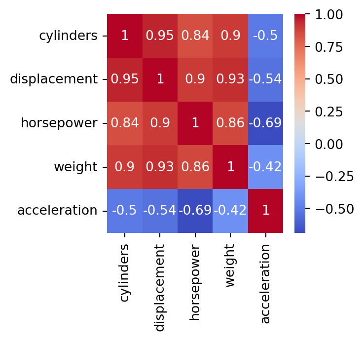
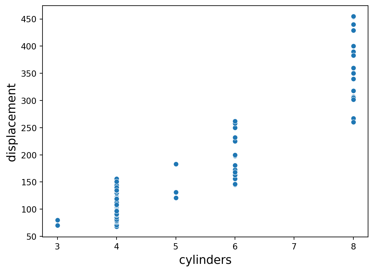
The predictors cylinders and displacement are highly correlated. In fact, their correlation is 0.95.
In practice
We deal with collinearity by removing the minimum number of predictors to ensure that all pairwise correlations are below a certain threshold, say, 0.75.
We can identify the variables that are highly correlated using quite complex code. However, here we will do it manually using the correlation map.
Standardizing predictors
Predictors with different units
Many good predictive models have issues with numeric predictors with different units:
Methods such as K-nearest neighbors are based on the distance between observations. If the predictors are on different units or scales, then some predictors will have a larger weight for computing the distance.
Other methods such as LASSO use the variances of the predictors in their calculations. Predictors with different scales will have different variances and so, those with a higher variance will play a bigger role in the calculations.
In a nutshell, some predictors will have a higher impact in the model due to its unit and not its information provided to it.
Standarization
Standardization refers to centering and scaling each numeric predictor individually. It puts every predictor on the same scale.
To center a predictor variable, the average predictor value is subtracted from all the values.
Therefore, the centered predictor has a zero mean (that is, its average value is zero).
To scale a predictor, each of its value is divided by its standard deviation.
Scaling the data coerce the values to have a common standard deviation of one.
In mathematical terms, we standardize a predictor as:
\[{\color{blue} \tilde{X}_{i}} = \frac{{ X_{i} - \bar{X}}}{ \sqrt{\frac{1}{n -1} \sum_{i=1}^{n} (X_{i} - \bar{X})^2}},\]
with \(\bar{X} = \sum_{i=1}^n \frac{x_i}{n}\).
Example 2 (cont.)
We use on the five numerical predictors in the complete_sbAuto dataset.
Two predictors in original units
Consider the complete_sbAuto dataset created previously. Consider two points in the plot: \((175, 5140)\) and \((69, 1613)\).
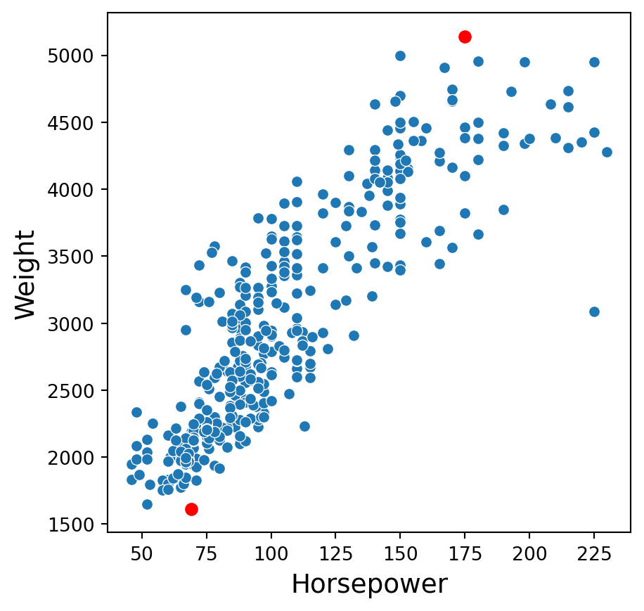
The distance between these points is \(\sqrt{(69 - 175)^2 + (1613-5140)^2}\) \(= \sqrt{11236 + 12439729}\) \(= 3528.592\).
Standarization in Python
To standardize numerical predictors, we use the function StandardScaler(). Moreover, we apply the function to the variables using the function fit_transform().
Unfortunately, the resulting object is not a pandas data frame. We then convert this object to this format.
| cylinders | displacement | horsepower | weight | acceleration | |
|---|---|---|---|---|---|
| 0 | 1.483947 | 1.077290 | 0.664133 | 0.620540 | -1.285258 |
| 1 | 1.483947 | 1.488732 | 1.574594 | 0.843334 | -1.466724 |
| 2 | 1.483947 | 1.182542 | 1.184397 | 0.540382 | -1.648189 |
| 3 | 1.483947 | 1.048584 | 1.184397 | 0.536845 | -1.285258 |
| 4 | 1.483947 | 1.029447 | 0.924265 | 0.555706 | -1.829655 |
Two predictors in standardized units
In the new scale, the two points are now: \((1.82, 2.53)\) and \((-0.91, -1.60)\).
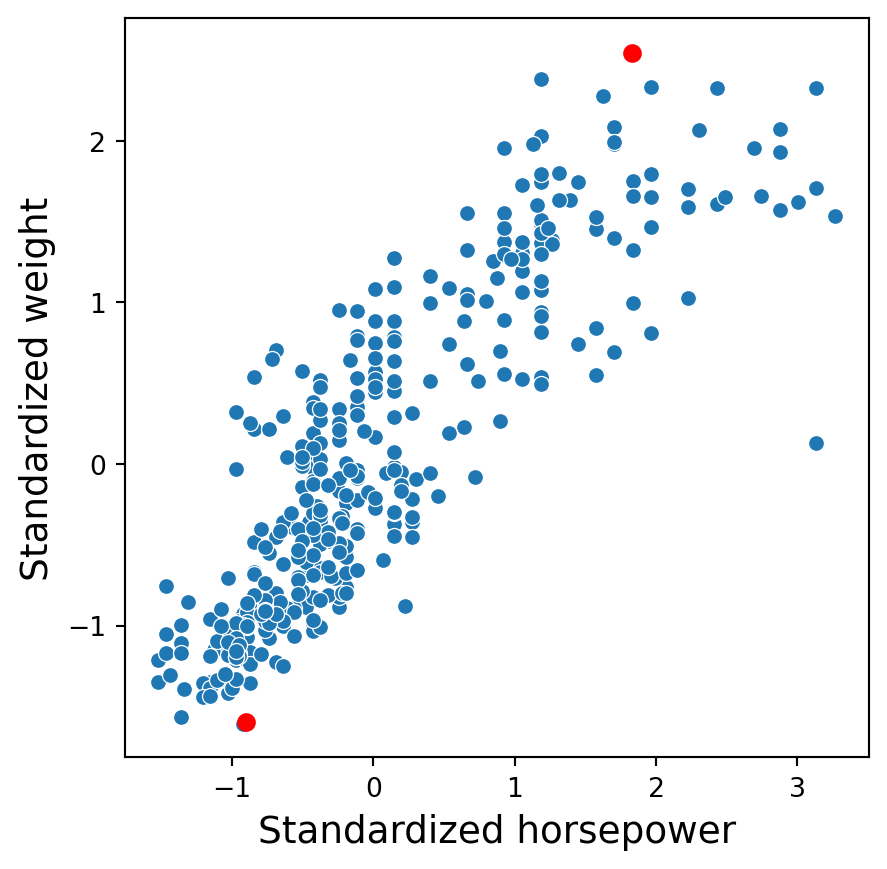
The distance between these points is \(\sqrt{(-0.91 - 1.82)^2 + (-1.60-2.53)^2}\) \(= \sqrt{7.45 + 17.05} = 4.95\).
Discussion
Standardized predictors are generally used to improve the numerical stability of some calculations.
It is generally recommended to always standardize numeric predictors. Perhaps the only exception would be if we consider a linear regression model.
A drawback of these transformations is the loss of interpretability since the data are no longer in the original units.
Standardizing the predictors does not affect their correlation.
Return to main page
![]()
Tecnologico de Monterrey